Lie symmetry analysis, conservation laws and diverse solutions of a new extended (2+1)-dimensional Ito equation

Ziying Qi; Lianzhong Li; Ziying Qi; Lianzhong Li

doi:10.3934/math.20231524

AIMS Mathematics

2023, Volume 8, Issue 12: 29797-29816. doi: 10.3934/math.20231524

Previous Article Next Article

Research article

Lie symmetry analysis, conservation laws and diverse solutions of a new extended (2+1)-dimensional Ito equation

Ziying Qi ,
Lianzhong Li ^,

School of Science, Jiangnan University, Wuxi 214026, China

Received: 04 September 2023 Revised: 30 September 2023 Accepted: 10 October 2023 Published: 02 November 2023
MSC : 76M60

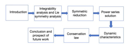
In this paper, a new class of extended (2+1)-dimensional Ito equations is investigated for its group invariant solutions. The Lie symmetry method is employed to transform the nonlinear Ito equation into an ordinary differential equation. The general solution of the solvable linear differential equation with different parameters is obtained, and the plot of the solvable linear differential equation is given. A power series solution for the equation is then derived. Furthermore, a conservation law for the equation is constructed by utilizing a new Ibragimov conservation theorem.

Keywords:

Citation: Ziying Qi, Lianzhong Li. Lie symmetry analysis, conservation laws and diverse solutions of a new extended (2+1)-dimensional Ito equation[J]. AIMS Mathematics, 2023, 8(12): 29797-29816. doi: 10.3934/math.20231524

Related Papers:

[1]	Miao Yang, Lizhen Wang . Lie symmetry group, exact solutions and conservation laws for multi-term time fractional differential equations. AIMS Mathematics, 2023, 8(12): 30038-30058. doi: 10.3934/math.20231536
[2]	Amjad Hussain, Muhammad Khubaib Zia, Kottakkaran Sooppy Nisar, Velusamy Vijayakumar, Ilyas Khan . Lie analysis, conserved vectors, nonlinear self-adjoint classification and exact solutions of generalized $ \left(N+1\right) $-dimensional nonlinear Boussinesq equation. AIMS Mathematics, 2022, 7(7): 13139-13168. doi: 10.3934/math.2022725
[3]	Farzaneh Alizadeh, Samad Kheybari, Kamyar Hosseini . Exact solutions and conservation laws for the time-fractional nonlinear dirac system: A study of classical and nonclassical lie symmetries. AIMS Mathematics, 2025, 10(5): 11757-11782. doi: 10.3934/math.2025532
[4]	A. Tomar, H. Kumar, M. Ali, H. Gandhi, D. Singh, G. Pathak . Application of symmetry analysis and conservation laws to a fractional-order nonlinear conduction-diffusion model. AIMS Mathematics, 2024, 9(7): 17154-17170. doi: 10.3934/math.2024833
[5]	Tamara M. Garrido, Rafael de la Rosa, Elena Recio, Almudena P. Márquez . Conservation laws and symmetry analysis of a generalized Drinfeld-Sokolov system. AIMS Mathematics, 2023, 8(12): 28628-28645. doi: 10.3934/math.20231465
[6]	Huizhang Yang, Wei Liu, Yunmei Zhao . Lie symmetry reductions and exact solutions to a generalized two-component Hunter-Saxton system. AIMS Mathematics, 2021, 6(2): 1087-1100. doi: 10.3934/math.2021065
[7]	Chaudry Masood Khalique, Oke Davies Adeyemo, Kentse Maefo . Symmetry solutions and conservation laws of a new generalized 2D Bogoyavlensky-Konopelchenko equation of plasma physics. AIMS Mathematics, 2022, 7(6): 9767-9788. doi: 10.3934/math.2022544
[8]	Mobeen Munir, Muhammad Athar, Sakhi Sarwar, Wasfi Shatanawi . Lie symmetries of Generalized Equal Width wave equations. AIMS Mathematics, 2021, 6(11): 12148-12165. doi: 10.3934/math.2021705
[9]	Yanxia Hu, Qian Liu . On traveling wave solutions of a class of KdV-Burgers-Kuramoto type equations. AIMS Mathematics, 2019, 4(5): 1450-1465. doi: 10.3934/math.2019.5.1450
[10]	Yuqiang Feng, Jicheng Yu . Lie symmetry analysis of fractional ordinary differential equation with neutral delay. AIMS Mathematics, 2021, 6(4): 3592-3605. doi: 10.3934/math.2021214

Abstract

1. Introduction

Nonlinear partial differential equations (NPDEs) are widely used to describe nonlinear phenomena in various disciplines, such as mechanics, control processes, ecological systems, economic systems, chemical cycle systems, and epidemiology ^[1,2,3,4,5]. The study of NPDEs is an important branch of modern mathematics, both in theory and practical applications. Finding exact solutions to NPDEs has been a central topic in mathematics and physics. In recent decades, mathematicians have developed several effective methods for finding structural solutions of NPDEs, including the Lie symmetry method^[6,7], Homogeneous equilibrium method^[8,9,10], Darboux transformation^[11], Bäcklund transformation^[12], F-expansion method^[13], Tanh method^[14,15], etc. Among these methods, Lie symmetry analysis is one of the most classical methods. It utilizes a set of one-parameter transformations in the space of independent and dependent variables to keep the NPDE unchanged. Lie symmetry methods have been widely applied to solve problems in mathematical physics, nonlinear science and engineering physics^[16,17,34]. It is well known that the famous (1+1)-dimensional the Ito equation is

$\begin{equation} u_{t t}+6u_{xx}u_t+6u_xu_{xt}+ u_{xxt} = 0. \end{equation}$

(1.1)

The above equation was firstly proposed by Ito, and its bilinear Bäcklund transform, Lax pair and multi-soliton solutions were obtained. The rolling behavior of a ship in regular sea is usually predicted by the Ito equation, and the interaction between two internal long waves can also be described by the Ito equation. Due to the typical nature of the Ito equation as a soliton equation, a great deal of research has been done concerning it. Ma and Li investigated the evolution and degradation of the torsional attractor solutions of the (2+1)-dimensional Hirota-satsuma-Ito class equations using symbolic computation and Hirota bilinear equations^[18]. Based on an extended homoclinic test and bilinear method, Li and Zhao studied the exact soliton solutions of the (2+1)-dimensional Ito equation and explicit solutions such as trigonometric function solution, soliton solution, double periodic wave solution and periodic solitary wave solution are obtained^[19]. Based on a multidimensional Bernhard Riemann $\xi$ function, Tian and Zhang used a clear and direct method to explicitly construct the periodic solutions of the (1+1)-dimensional and the (2+1)-dimensional Ito equations^[20]. Then, using Hirota's bilinear method and the positive quadratic function, Tian and Li obtained some global solutions of the (2+1)-dimensional Ito equation^[21].

Recently, Ma and Wu obtained the local interaction solution of the Ito equation with free parameters in the (2+1)-dimensional Ito equation by Hirota bilinear transformation^[22]. In 2022, based on previous studies ^[23,24,25], Wazwaz extended the equation to (3+1)-dimensional Ito equation, proved its complete integrability by Painleve analysis and derived the multi-soliton solution^[26] using the simplified Hirota method. Based on the traditional (2+1)-dimensional Ito equation,

$v_{t t}+v_{x x x t}+3\left(2 v_x v_t+v v_{x t}\right)+3 v_{x x} \int_{-\infty}^x v_t d x^{\prime}+\alpha v_{y t}+\beta v_{x t} = 0.$

Let $v = u_x$ , then the equation can be transformed to the following new form which is studied in this paper

$\begin{equation} u_{x tt}+u_{xxx xt}+3(2u_{xx}u_{xt}+u_xu_{xxt})+ 3u_{xxx}u_t+\alpha u_{x y t}+\beta u_{xxt} = 0, \end{equation}$

(1.2)

where $\alpha$ and $\beta$ are real parameters. The Ito equation is completely integrable and possesses many conservation laws. If $\beta = \alpha = 0$ , the above equation becomes (1+1)-dimensional. In this paper, Lie symmetry analysis method is used to study the Ito equation, some special solutions are found, their plots are drawn and dynamical behaviors are studied. The arrangement of this paper is shown in Figure 1 below.

Figure 1. The arrangement of the sections of this paper.

DownLoad: Full-Size Img PowerPoint

2. Integrability analysis and Lie symmetry analysis of the Ito equation

2.1. Integrability analysis of the Ito equation

Painlevé analysis ^[27] is a useful method for examining the complete integrability for NPDEs. We first assume that the solution of the equation is explored as

$u(x, y, t) = \sum\limits_{k = 0}^{\infty} u_k(x, y, t) \psi(x, y, t)^{k-\mu},$

which is a Laurent series with respect to a singular manifold $\psi(x, y, t)$ . Following the Painlevé analysis gives resonances at k = 1, 4 and 6. As a result, we obtain expressions for $u_2$ , $u_3$ and $u_5$ ,

$\begin{aligned} & u_2 = \beta \psi_t+\frac{\alpha^2}{2 \beta} t+\alpha^2 u_1, \\ & u_3 = u_1 \psi_t+\frac{\alpha}{2 \beta} t^2+\alpha^2\psi_x, \\ & u_5 = u_1 \psi_t+\alpha t\left(u_1 u_4+u_1^2\right)+\frac{\beta}{36\alpha^3} \psi_{y t}+u_4^2\psi_{xx}. \end{aligned}$

We found that $u_1$ , $u_4$ and $u_6$ are left as arbitrary functions and this confirms that Eq (1.2) passes the Painlevé test that confirms the complete integrability for Eq (1.2).

2.2. Lie symmetry analysis of the Ito equation

The one parameter Lie group of infinitesimal transformation of the Ito equation in $x$ , $y$ , $t$ and $u$ is given by

$\begin{aligned} &\tilde{x} \rightarrow x+\varepsilon \xi(x, y, t, u)+o\left(\varepsilon^{2}\right), \\ &\tilde{y} \rightarrow y+\varepsilon \phi(x, y, t, u)+o\left(\varepsilon^{2}\right), \\ &\tilde{t} \rightarrow t+\varepsilon \tau(x, y, t, u)+o\left(\varepsilon^{2}\right), \\ &\tilde{u} \rightarrow u+\varepsilon \eta(x, y, t, u)+o\left(\varepsilon^{2}\right), \end{aligned}$

where $\varepsilon$ is the group parameter. In particular, $\xi$ , $\phi$ , $\tau$ and $\eta$ are the infinitesimal operators of the transformation for the independent and dependent variables, which will be determined later. The vector field associated with the above mentioned group of transformations is given as

$\begin{equation} \begin{aligned} V = &\xi(x, y, t, u) \frac{\partial}{\partial x}+\phi(x, y, t, u) \frac{\partial}{\partial y} +\tau(x, y, t, u) \frac{\partial}{\partial t}+\eta(x, y, z, t, u) \frac{\partial}{\partial u}. \end{aligned} \end{equation}$

(2.1)

The symmetry group of Eq (1.2) will be generated by the vector field of the Eq (2.1). Using the invariant condition

$\begin{equation} \left.Pr^{5} V(\Delta)\right|_{\Delta = 0} = 0, \end{equation}$

(2.2)

where $\Delta = u_{x t t}+u_{x x x x t}+3\left(2 u_{x x} u_{x t}+u_x u_{x x t}\right)+3 u_{x x x} u_t+\alpha u_{x y t}+\beta u_{x x t}$ . The five-order prolongation for Eq (1.2) is

$\begin{aligned} Pr^{5} v = & v+\eta^x \frac{\partial}{\partial u_x}+\eta^t \frac{\partial}{\partial u_t}+\eta^{x x} \frac{\partial}{\partial u_{x x}}+\eta^{x t} \frac{\partial}{\partial u_{x t}}+\eta^{x x x} \frac{\partial}{\partial u_{x x x}}+\eta^{xtt} \frac{\partial}{\partial u_{x t t}} \\ & +\eta^{x x t} \frac{\partial}{\partial u_{x x t}}+\eta^{x y t} \frac{\partial}{\partial u_{x y t}}+\eta^{x x x x t} \frac{\partial}{\partial u_{x x x x t}}, \end{aligned}$

where

$\begin{aligned} & \eta^x = D_x\left(\eta-\xi u_x-\phi u_y-\tau u_t\right)+\xi u_{x x}+\phi u_{x y}+\tau u_{x t}, \\ & \eta^t = D_t\left(\eta-\xi u_x-\phi u_y-\tau u_t\right)+\xi u_{x t}+\phi u_{y t}+\tau u_{t t}, \\ & \eta^{x x} = D_x^2\left(\eta-\xi u_x-\phi u_y-\tau u_t\right)+\xi u_{x x x}+\phi u_{x x y}+\tau u_{x x}, \\ & \eta^{x t} = D_x D_t\left(\eta-\xi u_x-\phi u_y-\tau u_t\right)+\xi u_{x x t}+\phi u_{x y t}+\tau u_{x t t}, \\ & \eta^{x x x} = D_x^3\left(\eta-\xi u_x-\phi u_y-\tau u_t\right)+\xi u_{x x x}+\phi u_{x x y}+\tau u_{x x t}, \\ & \eta^{x t t} = D_x D_t^2\left(\eta-\xi u_x-\phi u_y-\tau u_t\right)+\xi u_{x xtt}+\phi u_{x y t t}+\tau u_{x t t t}, \\ & \eta^{x x t} = D_x^2 D_t\left(\eta-\xi u_x-\phi u_y-\tau u_t\right)+\xi u_{x x x t}+\phi u_{x x y t}+\tau u_{xtt}, \\ & \eta^{x y t} = D_x D_y D_t\left(\eta-\xi u_x-\phi u_y-\tau u_t\right)+\xi u_{x x y t}+\phi u_{x y y t}+\tau u_{x y t t}, \\ & \eta^{x x x x t} = D_x^4 D_t\left(\eta-\xi u_x-\phi u_y-\tau u_t\right)+\xi u_{x x x x x t}+\phi u_{x x x x y t}+\tau u_{x x xx tt}. \\ \end{aligned}$

Substituting these extensions in Eq (2.2), we get the determining equations:

$\begin{aligned} & \eta_x = -\frac{2}{9} \beta \phi_y+\frac{\alpha}{3} \xi_y, \eta_t = 0, \eta_u = -\frac{1}{3} \phi_y, \\ & \tau_x = \tau_u = 0, \tau_t = -\alpha\left(\tau_y\right)+\phi_y, \\ & \xi_u = \xi_t = 0, \xi_x = \frac{1}{3} \phi_y, \\ & \phi_u = \phi_x = \phi_t = 0 . \end{aligned}$

By using the software Maple to solve those equations, we get the following system of equations:

$\begin{aligned} & \xi = \frac{\left(F_{1 y}\right) x}{3}+F_3(y), \quad \phi = F_1(y), \quad\tau = \frac{F_2\left(\frac{\alpha t-y}{\alpha}\right) \alpha+F_1(y)}{\alpha} , \\ & \eta = \frac{\alpha\left(F_{1 y y}\right) x^2}{18}+\frac{(-4 \beta x-6 u)\left(F_{1 y }\right)}{18}+\frac{x \alpha\left(F_{3 y}\right)}{3}+F_4(y), \\ \end{aligned}$

where ${F_1}$ , ${F_3}$ and ${F_4}$ are arbitrary functions of $y$ and ${F_2}$ is a arbitrary function of $\frac{\alpha t-y}{\alpha}$ . In 2022, Kumar discussed a case where ${F_2}$ is a constant ^[28]. In this paper, we discuss the more general case. So we have

$F_1 = C_1y+C_8, \quad F_2 = C_2(\frac{\alpha t-y}{\alpha})+C_5, \quad F_3 = C_3y+C_6, \quad F_4 = C_4y+C_7,$

where $C_1$ , $C_2$ , $C_3$ , $C_4$ , $C_5$ , $C_6$ and $C_7$ are arbitrary constants. So the vector fields of equation (1.2) are

$\begin{aligned} & V_1 = \frac{\partial}{\partial x}, \quad V_2 = \frac{\partial}{\partial t}, \quad V_3 = \frac{\partial}{\partial u}, \quad V_4 = y\frac{\partial}{\partial u} , \quad V_5 = \left(t-\frac{y}{\alpha}\right) \frac{\partial}{\partial t}, \\ & V_6 = \frac{1}{\alpha} \frac{\partial}{\partial t}+\frac{\partial}{\partial y}, \qquad\qquad V_7 = \frac{\alpha}{3} x \frac{\partial}{\partial u}+y \frac{\partial}{\partial x} , \\ & V_8 = \frac{1}{18}(-4 \beta x-6 u) \frac{\partial}{\partial u}+\frac{y}{\alpha} \frac{\partial}{\partial t}+\frac{x}{3} \frac{\partial}{\partial x}+y \frac{\partial}{\partial y}.\\ \end{aligned}$

Thus, all the infinitesimals of Eq (1.2) can be written as the linear combination of the vectors $V_i$ as

$V = p_1 V_1+p_2 V_2+p_3 V_3+p_4 V_7+p_5 V_5+p_6 V_6+p_7 V_7+p_8V_8.$

The commutator relations of Lie algebra between the vector fields can be represented in Table 1.

Table 1. Commutator table.

*	$V_1$	$V_2$	$V_3$	$V_4$	$V_5$	$V_6$	$V_7$	$V_8$
$V_1$	$0$	$0$	$0$	$0$	$0$	$0$	$0$	$\frac{1}{3}V_1$
$V_2$	$0$	$0$	$0$	$0$	$0$	$V_2$	$0$	$0$
$V_3$	$0$	$0$	$0$	$0$	$0$	$0$	$0$	$-\frac{1}{3}V_3$
$V_4$	$0$	$0$	$0$	$0$	$-V_3$	$0$	$0$	$-\frac{4}{3}V_4$
$V_5$	$0$	$0$	$0$	$V_3$	$0$	$0$	$V_1$	$V_5$
$V_6$	$0$	$0$	$-V_2$	$0$	$0$	$0$	$0$	$0$
$V_7$	$0$	$0$	$0$	$0$	$-V_1$	$0$	$0$	$-\frac{2}{3}V_7-\frac{2}{9}\beta V_4$
$V_8$	$-\frac{1}{3}V_1$	$0$	$\frac{1}{3}V_3$	$\frac{4}{3}V_4$	$-V_5$	$0$	$\frac{2}{3}V_7$	$0$

| Show Table

DownLoad: CSV

To compute adjoint representations of symmetry operators for Eq (1.2), we use the Lie series^[29,30]

$A d\left(\exp \left(\vartheta \mathbb{V}_i\right)\right) \mathbb{V}_j = \sum\limits_{n = 0}^{\infty} \frac{\vartheta^n}{n !}\left(a d \mathbb{V}_i\right)^n\left(\mathbb{V}_j\right) = \mathbb{V}_j-\vartheta\left[\mathbb{V}_i, \mathbb{V}_j\right]+\frac{1}{2} \vartheta^2\left[\mathbb{V}_i, \left[\mathbb{V}_i, \mathbb{V}_j\right]\right]-\cdots.$

The full adjoint representation table entries are tabulated in Tables 2 and 3.

Table 2. Adjoint table.

Ad.	$V_1$	$V_2$	$V_3$	$V_4$
$V_1$	$V_1$	$V_2$	$V_3$	$V_4$
$V_2$	$V_1$	$V_2$	$V_3$	$V_4$
$V_3$	$V_1$	$V_2$	$V_3$	$V_4$
$V_4$	$V_1$	$V_2$	$V_3$	$V_4$
$V_5$	$V_1$	$V_2$	$V_3$	$V_4-\varepsilon V_3$
$V_6$	$V_1$	$V_2+V_2ln(\varepsilon+1)$	$V_3$	$V_4$
$V_7$	$V_1$	$V_2$	$V_3$	$V_4$
$V_8$	$V_1-V_1ln(1-\frac{1}{3}\varepsilon)$	$V_2$	$V_3-V_3ln(\frac{1}{3}\varepsilon+1)$	$V_8$

| Show Table

DownLoad: CSV

Table 3. Adjoint table.

Ad.	$V_5$	$V_6$	$V_7$	$V_8$
$V_1$	$V_5$	$V_6$	$V_7$	$V_8-\frac{1}{3}\varepsilon V_1$
$V_2$	$V_5$	$V_6-\varepsilon V_2$	$V_7$	$V_8$
$V_3$	$V_5$	$V_6$	$V_7$	$V_8+\frac{1}{3}\varepsilon V_3$
$V_4$	$V_5+\varepsilon V_3$	$V_6$	$V_7$	$V_8+\frac{4}{3}\varepsilon V_4$
$V_5$	$V_5$	$V_6$	$V_7-\varepsilon V_1$	$V_8-\varepsilon V_5$
$V_6$	$V_5$	$V_6$	$V_7$	$V_8$
$V_7$	$V_5+\varepsilon V_1$	$V_6$	$V_7$	$(1+\frac{2}{3}\varepsilon)V_7+\frac{2}{9}\varepsilon V_4$
$V_8$	$\varepsilon V_5$	$V_6$	$V_7-V_7ln(\frac{2}{3}\varepsilon+1)$	$V_8$

| Show Table

DownLoad: CSV

With the assistance of Tables 1, 2 and 3, by carefully applying adjoint maps, we discuss useful linear combinations of vector fields for the considered equation, which are taken as follows:

${({\rm{i}}) V_1+V_3+V_6 , \qquad({\rm{ii}}) V_1+V_4+V_6 , \qquad({\rm{iii}}) V_2+V_7 , \qquad({\rm{iv}}) V_8. }$

3. Similarity reduction of the Ito equation

In this section, we obtain numerous closed-form invariant solutions for equation (1.2) utilizing the Lie symmetry analysis. Two stages of symmetry reducations will be taken with the aid of invariant (or similarity) functions. We firstly solve the associated Lagrange's characteristic system given by

$\frac{d x}{\xi} = \frac{d y}{\phi} = \frac{d t}{\tau} = \frac{d u}{\eta},$

which leads to similarity functions.

3.1. Symmetry reduction for $V_{1}+V_{3}+V_{6}=\frac{\partial}{\partial x}+\frac{\partial}{\partial y}+\frac{1}{\alpha} \frac{\partial}{\partial t}+\frac{\partial}{\partial u}$

We use the symmetry $V_1+V_3+V_6$ to reduce the Ito equation (1.2) to a nonlinear partial differential equation (NODE). The characteristic equations of $V_1+V_3+V_6$ give the invariants

$\begin{equation} T = -\alpha t+y, \quad X = -\alpha t+x , \quad V = -\alpha t+u. \end{equation}$

(3.1)

Replacing Eq (1.2) with Eq (3.1), we obtain the reduced (1+1)-dimensional equation:

$\begin{equation} \begin{aligned} & (\alpha-\beta) V_{X X T}+(\alpha-\beta) V_{X X X}-V_{X X X X X}-V_{X X X XT}-6 V_{X X} V_{X T}-6 V_{X X}^2\\ &-6 V_X V_{X X X}-3 V_X V_{X X T}-3 V_T V_{X X X} = 0. \end{aligned} \end{equation}$

(3.2)

Then we apply the classical symmetry again, the vector fields of Eq (3.2) are

$\begin{aligned} & \bar{V}_1 = \frac{1}{3}[(-2 T+2 X) \alpha+(2 T-2 X) \beta-3 V] \frac{\partial}{\partial V}+T \frac{\partial}{\partial T}+X \frac{\partial}{\partial X}, \\ & \bar{V}_2 = \frac{\partial}{\partial T} , \qquad\bar{V}_3 = \frac{\partial}{\partial V} , \qquad \bar{V}_4 = T \frac{\partial}{\partial T}+T \frac{\partial}{\partial X}. \end{aligned}$

3.1.1. For $\bar{V}_1$

We obtain the invariants

$w = \frac{X}{T} , R = \left[V+\left(\frac{\alpha}{3}-\frac{\beta}{3}\right) T-\left(\frac{\alpha}{3}-\frac{\beta}{3}\right) X \right] T .$

By substituting group invariant solution, we have the reduced equation

$\begin{equation} 6(w-1) R_w R_{w w w}+6(w-1) R_{w w}^2+(w-1) R_{w w w w w}+21 R_w R_{w w}+3 R_{w w w} R_{w w} = 0. \\ \end{equation}$

(3.3)

The exact solutions of equation (3.3) have been found in Section 4.1.

3.1.2. For $\bar{V_2}+\bar{V_3}+\bar{V_4}$

We obtain the invariants

$\begin{aligned} w = -T+\ln (T+1)+X, R = V-\ln (T+1), \end{aligned}$

which reduce Eq (3.2) to a NODE

$(\alpha-\beta) R_{w w w}-R_{w w w w w}-6 R_{w w}^2-6 R_w R_{w w w} = 0. \\$

Obviously, the general solution is not easy to find so we obtain a particular solution

$\begin{equation} u = -\tan \left(\frac{\alpha x-y+\ln y}{2}+1\right)+3+\beta\ln y .\\ \end{equation}$

(3.4)

3.2. Symmetry reduction for $V_1+V_4+V_6=y \frac{\partial}{\partial u}+\frac{1}{\alpha} \frac{\partial}{\partial t}+\frac{\partial}{\partial y}+\frac{\partial}{\partial x}$

We use the symmetry $V_1+V_4+V_6$ to reduce equation (1.2) to a NODE. The characteristic equations give the similar invariants

$X = -\alpha t+x, \quad T = -\alpha t+y, \quad V = u+\frac{1}{2} \alpha^2 t^2-\alpha ty .\\$

By substituting the group invariant solution, we have the reduced equation

$\begin{equation} \begin{aligned} &(\alpha-\beta) V_{X X T}+(\alpha-\beta+3 T) V_{X X X}-V_{X X X X X}-V_{X X X X T} \\ &-6 V_{X X}^2-6 V_{X X} V_{X T}-3 V_X V_{X X T}-6 V_X V_{X X}-3 V_T V_{X X X} = 0. \end{aligned} \end{equation}$

(3.5)

In order to simplify the equation further, we use Maple to analyze Eq (3.5) for the second Lie symmetry have the vector fields,

$\begin{aligned} & \bar{V}_1 = \left[9 T^2+(4 \beta-4 \alpha)(T-X)-6 V \right] \frac{\partial}{\partial V}+6T \frac{\partial}{\partial T}+6 X \frac{\partial}{\partial X} , \quad\bar{V}_3 = \frac{\partial}{\partial V}, \\ & \bar{V}_2 = T \frac{\partial}{\partial V}+\frac{\partial}{\partial T} , \qquad\bar{V}_4 = T^2 \frac{\partial}{\partial V}+T \frac{\partial}{\partial T}+T \frac{\partial}{\partial X}.\\ \end{aligned}$

3.2.1. For $\bar{V}_1$

We obtain the similarity variable in the same way as follows:

$w = \frac{X}{T} , \quad R = \left[V-\frac{T^2}{2}+\left(\frac{\alpha}{3}-\frac{\beta}{3}\right) (T- X)\right] T.$

Then we obtain the following reduced equation:

$\begin{equation} (w-1) R^{(5)}+5 R^{(4)}+6(w-1) R_{w w}^2+21 R_w R_{w w}+6(w-1) R_w R_{w w w}+3 R R_{w w w} = 0. \end{equation}$

(3.6)

The exact solutions of equation (3.6) have been found in Section 4.2.

3.2.2. For $\bar{V}_2$

We obtain the similarity variable in the same way as follows:

$w = X , \qquad R = V-\frac{T^2}{2}.$

Then we get following reduced equation:

$(\alpha-\beta+3 T) R_{w w w}-R_{w w w w w}-6 R_{w w}^2-6 R_w R_{w w w}-3 T R_{w w w} = 0. \\$

By simple calculation, we find a solution for equation (1.2)

$\begin{equation} u = -\frac{1}{2} \tanh \left(\frac{\alpha t-x}{2}\right)^2+\frac{1}{2} y^2+\frac{1}{2}. \\ \end{equation}$

(3.7)

3.2.3. For $\bar{V}_2+\bar{V}_3+\bar{V}_4$

We obtain the similar variable invariants by solving the characteristic equation,

$w = X+\ln (T+1)-T , \quad R = V-\frac{T^2}{2}-\ln (T+1). \\$

Then we have the reduced equation

$(\alpha-\beta) R_{w w w}-R_{w w w w w}-6 R_w^2-6 R_w R_{w w w} = 0 .\\$

By simple calculation, we can obtain the group invariant solution of the equation (1.2)

$\begin{equation} u = -\tan \left(\frac{x-y+\ln (-\alpha t+y+1)}{2}+\frac{1}{2}\right)+\frac{1}{2}+\frac{1}{2} y^2+\ln (-\alpha t+y+1). \\ \end{equation}$

(3.8)

3.3. Symmetry reduction for $V_2+V_7=\frac{\alpha}{3} x \frac{\partial}{\partial u}+y \frac{\partial}{\partial x}+\frac{\partial}{\partial t}$

Solving the characteristic equation, we obtain the similarity variables and function

$T = -t y+x , \quad Y = y, \quad V = u+\frac{\alpha}{6} y t^2-\frac{\alpha}{3} t x.$

Now, substituting the values of the similarity variables in Eq (1.2), we obtain the reduced (1+1)-dimensional equation as follows:

$\begin{equation} \left(Y^2+\alpha T-\beta Y\right) V_{T T T}-Y V_{T T TTT}-6 Y V_{T T}^2-\alpha V_{T T}-\alpha Y V_{T T Y} = 0 . \end{equation}$

(3.9)

Again applying similarity transformation method (STM) on Eq (3.9), we get the following results:

$\begin{aligned} \bar{V}_1 = 3V \frac{\partial}{\partial V}+\left( 3T+\frac{Y(3 \beta-5 Y)}{\alpha}\right) \frac{\partial}{d T}+9 Y \frac{\partial}{d Y} , \quad\bar{V}_2 = \frac{1}{Y} \frac{\partial}{\partial T}. \end{aligned}$

3.3.1. For $\bar{V_1}$

We obtain the similarity variable as follows:

$w = \frac{6\alpha T +2 Y^2-3 \beta Y}{6 \alpha Y^{\frac{1}{3}}} , R = \frac{V}{Y^{\frac{1}{3}}} .\\$

Now, we have the following equation by substituting:

$\begin{equation} 4 \alpha w R_{w w w}-3 R_{w w w w w}-18 R_{w w}^2-2 \alpha R_{w w} = 0. \\ \end{equation}$

(3.10)

The exact solutions of equation (3.10) have been found in Section 4.

3.4. Symmetry reduction for $V_8=\frac{1}{18}(-4 \beta x-6 u) \frac{\partial}{\partial u}+\frac{y}{\alpha} \frac{\partial}{\partial t}+\frac{x}{3} \frac{\partial}{\partial x}+y \frac{\partial}{\partial y}$

The characteristic equations of $V_8$ give the similar invariants

$\begin{equation} \begin{aligned} X = x y^{-\frac{1}{3}} , \quad T = -\alpha t+y , \quad V = \left(u+\frac{\beta x}{3}\right) y^{\frac{1}{3}}, \\ \end{aligned} \end{equation}$

(3.11)

we put Eq (3.11) into Eq (1.2) and get the following reduced equation:

$-3 V_{X X X X T}-18 V_{X X} V_{X T}-9 V_{XXT} V_X-9 V_{X X X} V_T+X V_{X X T}+2 \alpha V_{X T} = 0.$

Since the above equation contains one dependent and two independent variables, we again apply the STM. Thus the Lie algebra of the above equation is spanned by the following vector fields

$\begin{aligned} \bar{V}_1 = \frac{1}{9} X \frac{\partial}{\partial V}+\frac{\partial}{\partial X}, \qquad\bar{V}_2 = \frac{\partial}{\partial V}, \qquad\bar{V}_3 = T \frac{\partial}{\partial T}.\\ \end{aligned}$

3.4.1. For $\bar{V_1}+\bar{V_3}$

We obtain the similarity variable as follows:

$w = -\ln T+X , \quad R = V+\frac{\ln ^2 T}{18}-\frac{X \ln T}{9}. \\$

By substituting, we obtain the reduced equation as:

$\begin{equation} -3 R^{(5)}+18\left(R_{w w}\right)^2-2(\alpha+1) R_{w w}+18 R_w R_{w w w}-2 w R_{w w w}+\frac{2 \alpha}{9} = 0. \\ \end{equation}$

(3.12)

The exact solutions of equation (3.12) have been found in Section 4.

3.4.2. For $\bar{V}_2+\bar{V}_3$

We obtain the similarity variable as follows:

$w = X , \quad R = V-\ln T. \\$

Similarly, we obtain the reduced equation by substituting:

$\quad-9 \frac{1}{T} R_{w w w} = 0.$

By simple calculation, we obtain a solution of equation (1.2)

$\begin{equation} u = -\frac{\beta}{3} x+y^{-\frac{1}{3}} \ln (-\alpha t+y)+a_0 y^{-\frac{1}{3}}+a_1 x y^{-\frac{2}{3}}+a_2 x^2 y^{-1} . \\ \end{equation}$

(3.13)

4. Exact explicit solutions of reduction equation

The solutions of nonlinear ordinary differential equations cannot be expressed by elementary functions. So we assume that the power series solution of equation (1.2) is

$\begin{equation} R(w) = \sum\limits_{n = 0}^{\infty} a_n w^n. \\ \end{equation}$

(4.1)

$\begin{equation} \begin{aligned} & R^{\prime} = \sum\limits_{n = 0}^{\infty}(n+1) a_{n+1} w^n, \\ & R^{\prime \prime} = \sum\limits_{n = 0}^{\infty}(n+1)(n+2) a_{n+2} w^n, \\ &\left(R^{\prime \prime}\right)^2 = \sum\limits_{n = 0}^{\infty} \sum\limits_{i = 0}^n(i+1)(i+2)(n+1)(n+2) a_{n+2} a_{i+2} w^{n+i}, \\ & R^{\prime \prime \prime} = \sum\limits_{n = 0}^{\infty}(n+1)(n+2)(n+3) a_{n+3} w^n, \\ & R^{(4)} = \sum\limits_{n = 0}^{\infty}(n+1)(n+2)(n+3)(n+4) a_{n+4} w^n, \\ & R^{(5)} = \sum\limits_{n = 0}^{\infty}(n+1)(n+2)(n+3)(n+4)(n+5) a_{n+5} w^{n } . \end{aligned} \end{equation}$

(4.2)

4.1. The power series solution of Eq (3.3)

Substituting Eq (4.1) and Eq (4.2) into Eq (3.3) and comparing coefficients, we have

$a_5 = \frac{7}{20} a_1 a_2+\frac{3}{10} a_2 a_3-\frac{3}{10} a_1 a_3-\frac{1}{5} a_2^2.$

Consider $n \geq 1$ , we get

$\begin{aligned} a_{n+5}& = \frac{1}{(n+1)(n+2)(n+3)(n+4)(n+5)}\left[6 \sum\limits_{i = 0}^n \sum\limits_{j = 0}^i(j+1)(i+1)(i+2)(i+j) a_{i+2} a_{i+1} \right.\\ & \left.-6 \sum\limits_{i = 0}^n \sum\limits_{j = 0}^i(j+1)(i+1)(i+2)(i a_{j+1} a_{i+3}+3 a_{j+1} a_{i+3}+j a_{i+2} a_{j+2}+2 a_{i+2} a_{j+2}) \right.\\ \end{aligned}$

$\begin{aligned} & \left.+\sum\limits_{i = 0}^n i(i+1)(i+2)(i+3)(i+4) a_{i+4}+3 \sum\limits_{i = 0}^n \sum\limits_{j = 0}^i(j+1)(j+2)(i+1)[(i+2)(i+3) a_{i+3}\right.\\ &\left.+7 a_{i+1}] a_{j+2}\right].\\ \end{aligned}$

From the above recurrence formula, the coefficients of the power series solution can be determined by $a_1$ , $a_2$ , $a_3$ and $a_4$ , then the power series solution of Eq (3.3) can be written as:

$R(w) = a_0+a_1 w+a_2 w^2+a_3 w^3+a_4 w^4+a_5 w^5+\sum\limits_{n = 1}^{\infty} a_{n+5} w^{n+5}.\\$

Thus, we obtain the exact power series solution of Eq (1.2) as follows:

$\begin{equation} \begin{aligned} u = &\frac{1}{(-\alpha t+y)}\left[a_0+a_1\left(\frac{-\alpha t+x}{-\alpha t+y}\right)+a_2\left(\frac{-\alpha t+x}{-\alpha t+y}\right)^2+a_3\left(\frac{-\alpha t+x}{-\alpha t+y}\right)^3+a_4\left(\frac{-\alpha t+x}{-\alpha t+y}\right)^4\right. \\ & \left.+a_5\left(\frac{-\alpha t+x}{-\alpha t+y}\right)^5+\sum\limits_{n = 1}^{\infty} a_{n+5}\left(\frac{-\alpha t+x}{\alpha t+y}\right)^{n+5}\right]+\alpha t-\frac{1}{3}(\alpha-\beta)(y-x). \\ \end{aligned} \end{equation}$

(4.3)

Next, the convergence of the solution is considered

$\begin{aligned} a_{n+5} \leq & \left|\frac{1}{(n+1)(n+2)(n+3)(n+4)(n+5)}\right|\left[\sum\limits_{i = 0}^n(i+1)(i+2)(i+3)(i+4)(i+5)\left|a_{i+4}\right|\right. \\ & +\sum\limits_{i = 0}^n \sum\limits_{j = 0}^i(i+1)(i+2)(j+1)(6 i+21)\left|a_{j+1}\right|\left|a_{i+2}\right|+\sum\limits_{i = 0}^n \sum\limits_{j = 0}^i(i+1)(i+2)(i+3) \\ & \left.|3 a_j-6 a_{j+1}(j+1)\right|\left|a_{i+3}\right|+6 \sum\limits_{i = 0}^n \sum\limits_{j = 0}^i (j+1)(j+2)(i+1)|i a_{i+1}-i a_{i+2}-2 a_{i+2}||a_{j+2}| \\ \leq & M[\sum\limits_{i = 0}^n\left|a_{i+4}\right|+\sum\limits_{i = 0}^n \sum\limits_{j = 0}^i|a_{i+2}||a_{j+1}| \end{aligned}$

where $M\geq 1$ . Then we set up a new power series of the form $P(z) = \sum_{n = 0}^{\infty} b_n z^n$ , where $b_0 = |a_0|$ , $b_1 = |a_1|$ , $b_2 = |a_2|$ , $b_3 = |a_3|$ , $b_4 = |a_4|$ and

$b_{n+5} = M\left[\sum\limits_{i = 0}^n b_{i+4}+\sum\limits_{i = 0}^n \sum\limits_{j = 0}^i b_{i+2} b_{j+1}\right], n = 0, 1, 2\cdot\cdot\cdot.$

Obviously, we can get $|a_n|\leq b_n$ , $n = 0, 1, 2, 3, \cdot \cdot \cdot$ . In other words, the constructed power series $P(z)$ is a superior series of $R(w)$ . So

$P(z) = b_1 z+b_2 z^2+b_3 z^3+b_4 z^4+b_5 z^5+M \sum\limits_{n = 1}^{N_i} \sum\limits_{i = 0}^n[b_{i+4}+\sum\limits_{j = 0}^i b_{i+2} b_{j+2}+] z^{n+5}.$

Now, we construct an implicit function of $z$

$F(z, P) = P-b_0-b_2 z-b_2 z^2-b_3 z^3-b_4 z^4-b_5 z^5-M z^5\left(P \pm P^{\prime} P^{\prime \prime}\right)$

$F$ is analytic in $(0, b_0)$ , so $F(0, b_0)$ and $\frac{\partial}{\partial b} F\left(0, b_0\right) \neq 0$ . According to the implicit function theorem, we prove that the solution of this equation is convergent.

4.2. The power series solution of Eq (3.6)

For Eq (3.6), we get in the same way

$\begin{aligned} &a_5 = a_4-\frac{1}{20}\left(4 a_4^2-7 a_1 a_2+3 a_0 a_3+6 a_1 a_3\right), \\ &a_{n+5} = \frac{1}{(n+1)(n+2)(n+3)(n+4)(n+5)}\left[\sum\limits_{i = 0}^n(i+1)(i+2)(i+3)(i+4)(i+5) a_{i+4} .\right. \\ & +\sum\limits_{i = 0}^n \sum\limits_{j = 0}^i(i+1)(i+2)(j+1) a_{j+1} a_{i+2}(6 i+21)+\sum\limits_{i = 0}^n \sum\limits_{j = 0}^i(i+1)(i+2)(i+3) a_{i+3} \\ & \left.\left[3 a_j-6 a_{j+1}(j +1)\right]+6 \sum\limits_{i = 0}^n \sum\limits_{j = 0}^i(j+1)(j+2)(i+1) a_{j+2}\left(i a_{i+1}-i a_{i+2}-2 a_{i+2}\right)\right].\\ \end{aligned}$

Thus, the particular solution of Eq (1.2) is

$\begin{equation} \begin{aligned} u = &\frac{1}{-\alpha t+y}[a_0+a_1(\frac{-\alpha t+x}{-\alpha t+y})+a_2(\frac{-\alpha t+x}{-\alpha t+y})^2+a_3(\frac{-\alpha t+x}{-\alpha t+y})^3+a_4(\frac{-\alpha t+x}{-\alpha t+y})^4+a_5(\frac{-\alpha t+x}{-\alpha t+y})^5\\ & +\sum\limits_{n = 1}^{\infty} a_{n+5}(\frac{-\alpha t+x}{-\alpha t+y})^{n+5}]-\frac{1}{2} \alpha^2 t^2+\alpha t y+\frac{(-\alpha t+y)^2}{2}-\frac{1}{3}(\alpha-\beta)(y-x). \end{aligned} \end{equation}$

(4.4)

Similar to the convergence analysis method of solution (4.3), we can also obtain the convergence of solution (4.4). Similar to the above method, we also obtain the power series solutions for Eq (3.10) and Eq (3.12). The results will not be repeated.

5. Dynamical characteristics

In this section, we will analyze the dynamical behavior of the solutions derived in the previous section with three-dimensional and corresponding contour plots for the (2+1)-dimensional Ito equation when parameters take different values.

5.1. Three-dimensional and contour plots of the solution (3.4)

In 3.1.2, we have obtained a solution (3.4) to the (2+1)-dimensional Ito equation,

$u = -\tan \left(\frac{x-y+\ln y}{2}+1\right)+3+\ln y.\\$

Clearly, we find that $u$ is independent of time t. Then we have $\beta = 1$ and observe the dynamics of $u_{1}$ when $\alpha$ varies. With the help of Maple, the physical properties and characteristics of the solution are clearly depicted in Figures 2 and 3.

Figure 2. Three-dimensional plots of solution (3.4) with arbitrary constants

$\alpha = 1, 2, 3$ ,

$\beta = 1$ .

DownLoad: Full-Size Img PowerPoint

Figure 3. 2D-contour plots of solution(3.4) with arbitrary constants

$\alpha = 1, 2, 3$ ,

$\beta = 1$ .

DownLoad: Full-Size Img PowerPoint

The three-dimensional graphs represent the local structure, while the contour plots show the wave fluctuations. The denser the location in the plot, the greater the fluctuation. We observe the interaction of (3.4) at $\alpha = 1, 2, 3$ , and this change alters the speed, amplitude and shape of the wave so that there are more points of aggregation and the image becomes more dense when $\alpha$ increases. In Eq (1.2), parameter $\alpha$ is the coefficient of $u_{xyt}$ , parameter $\beta$ is the coefficient of $u_{xxt}$ , and we fixed the value of $\beta$ and took different values for $\beta$ . We found that the amplitude and shape of the wave did not change significantly, but the motion of the wave accelerated, making the wave in the plot more dense, which can be understood in a physical sense. As the interaction effect of the two internal long waves increases, the rolling behavior of the ship in the common sea area is accelerated.

5.2. Three-dimensional and contour plots of the solution (3.8)

In 3.2.3, we have obtained the group invariant solution (3.8) of the Eq (1.2),

$u = -\tan \left(\frac{x-y+\ln (-\alpha t+y+1)}{2}+\frac{1}{2}\right)+\frac{1}{2}+\frac{1}{2} y^2+\ln (-\alpha t+y+1).$

With the help of Maple, the three-dimensional dynamic graphs of the wave married with corresponding contour plots were depicted in and , and we directly observe the interaction phenomena of the solutions at times $t = -5, 0, 2$ . At first, the distribution of aggregation points is more scattered, then the aggregation points gradually increase and the wave spreads and continues to move. For Eq (3.8), where the interaction parameters of two internal long waves are fixed, which is the values of arbitrary constants $\alpha$ and $\beta$ , we discuss the dynamic behavior of the wave with respect to $t$ . With the increase of $t$ , the amplitude and shape of a single wave does not change significantly, and the frequency of the wave first decreases and then increases. At $t = 0$ , the frequency of the wave is the smallest. Then, we also found that the equilibrium position of the fluctuations increased significantly over time. From a physical point of view, we believe that over time, there is a clear upward trend in the equilibrium position of ships where rolling behavior occurs in common sea areas.

Figure 4. Three-dimensional plots of solution (3.8) at

$t = -5, 0, 2$ ,

$\alpha = 1$ .

DownLoad: Full-Size Img PowerPoint

Figure 5. 2D-contour plots of solution (3.8) at

$t = -5, 0, 2$ ,

$\alpha = 1$ .

DownLoad: Full-Size Img PowerPoint

6. Conservation laws of the Ito equation

This section describes a new conservation law proposed by Ibragimov^[5,31,32,33] for the Ito equation, which is necessary for testing the integrability and the existence and uniqueness of the solutions. The conservation laws hoids that

$D_x C^x+D_y C^y+D_t C^t = 0,$

where $D_{i}$ is the total derivative operator

$\begin{aligned} D_i = \frac{\partial}{\partial x^i}+u_{i} \frac{\partial}{\partial u}+s_i \frac{\partial}{\partial s}+u_{i j} \frac{\partial}{\partial u_j}+s_{i j} \frac{\partial}{\partial s_j}+u_{i j k} \frac{\partial}{\partial u_{j k}}+s_{i j k} \frac{\partial}{\partial S_{j k}}+\cdots \cdots. \end{aligned}$

The Ito equation has the formal Lagrangian

$\begin{equation} L = s(x, y, t)\left[u_{x t t}+u_{x x x t}+6 u_{x x} u_{x t}+3 u_x u_{x x t}+3 u_{x x} u_t+\alpha u_{x y t}+\beta u_{x x t}\right] . \\ \end{equation}$

(6.1)

From (6.1), we have

$\begin{aligned} & \frac{\partial L}{\partial u_x} = 3 s u_{x t}, \quad \quad \frac{\partial L}{\partial u_t} = 3 s u_{x x x}, \quad \frac{\partial L}{\partial u_{t t}} = 6 s u_{x x}, \quad \frac{\partial L}{\partial u_{x x}} = 6 s u_{x t}, \\ & \frac{\partial L}{\partial u_{x t}} = s, \quad \frac{\partial L}{\partial u_{x x t}} = (3 u_x+\beta) s, \quad \frac{\partial L}{\partial u_{x x}} = 3 s u_t, \quad \frac{\partial L}{\partial u_{x y}} = \alpha s.\\ \end{aligned}$

The adjoint equation of the Ito equation is expressed as

$F^* = 3 s_x u_{x x t}-3 s_{x x} u_{x t}-s_{x t t}-3 s_{x x t} u_x-3 s_{x x} u_{x x t} -3 s_x u_{x x x t}-\beta s_{x x t}-3 s_{x x x} u_t-\alpha s_{x y t}-s_{x x x x x t}. \\$

Since the Ito equation is nonlinear and self-adjoint, let u = s and we have

$-3 u_{x x} u_{x t}-u_{x t t}-3 u_{x x} u_{x x t}-3 u_x u_{x x x t}-\beta u_{x x}-3 u_{x x x} u_t-\alpha u_{x y t}-u_{x x x t} = 0.\\$

Therefore, we observe that Eq (1.2) is not fully recovered. Thus, Eq (1.2) is not self-adjoint. Now, the conserved vectors are given by

$\begin{aligned} C^x& = \xi_x L+W[u_{x x t}\left(3 s-9 s_x\right)+6 u_{x t}\left(s_x-s_{x x}\right)-6 s u_{x x x t}-3 s_t u_{x x}+(3 u_x+\beta) s_{x t}+s_{t t}\\ &+3 s_{x x} u_t+\alpha s_{y t}+s_{x x x t}] +W_x(-3 s_t u_x-\beta s_t-3 s_x u_t-s_{x x t})-\alpha W_y s_t+W_t (3 su_{x x}-s_t\\ &-3 u_x s_x-\beta s_x-\alpha s_y-s_{x x x}) +W_{x x}\left(3 s u_t+s_{x t}\right)+W_{x t}\left(3 s u_x+\beta s+s_{x x}\right) +\alpha W_{y t} s \\ & +W_{t t} s-W_{x x} s_t-W_{x x} s_x+W_{x x x} s , \\ \end{aligned}$

$\begin{aligned} C^y& = \xi_y L+\alpha W s_{x t}-\alpha W_x s_t-\alpha W_t s_x+W_{x t} s , \\ C^t& = \tau L+W(s_{x t}+3 u_x s_{x x}+\beta s_{x x}+\alpha s_{x y}+s_{x x x x x})+W_x(3 s_{u_x}-s_t-3 u_x s_x-\beta s_x-\alpha s_y \\ & -s_{x x x})-\alpha W_y s_x-W_t s_x +W_{x x}(3 s u_x+\beta s+s_{x x})+W_{x x} s+\alpha W_{x y} s-W_{x x} s_x+W_{x x x x} s. \\ \end{aligned}$

with $W = \eta-\xi u_x-\phi u_y-\tau u_t$ . These equations contain arbitrary function $s(x, y, t)$ , arbitrary parameters $\alpha$ and $\beta$ . This leads to the generation of an infinite number of conservation laws by defining their conservation vectors. Therefore, we can write the conservation laws for the vector fields (ⅰ)–(ⅳ) in this way.

6.1. For $V_1+V_3+V_6=\frac{\partial}{\partial x}+\frac{\partial}{\partial y}+\frac{1}{\alpha} \frac{\partial}{\partial t} +dy \frac{\partial}{\partial u}$

For vector field $V_1+V_3+V_6$ , we have $W = dy- u_x- u_y-\frac{1}{\alpha}u_t$ .

$\begin{aligned} C^x& = s(u_{x t t}+u_{x x x x t}+6 u_{x x} u_{x t}+3 u_x u_{x x t}+3 u_{x x x} u_t+\alpha u_{x y t}+\beta u_{x x t})+(dy-u_x-u_y \\ & -\frac{1}{\alpha} u_t)(3 su_{x x t}-6 s_{x x} u_{x t}-9 s_x u_{x x t}-6 su_{x x xt}-3 s_t u_{x x} +3 s_{x t} u_x+\beta s_{x t}+s_{tt}+3 s_{x x } u_t\\ & +6 s_x u_{x t}+\alpha s_{y t}+s_{x x x t})+(u_{x x}+u_{x y} +\frac{1}{\alpha} u_{x t})(3 s_t u_x+\beta s_t+3 s_x u_t+s_{xxt})-\alpha s_t(d\\ & -u_{x y}-u_{y y}-\frac{1}{\alpha} u_{y t}) +(-u_{x t}-u_{y t}-\frac{1}{\alpha} u_{t t})(3 su_{xx}-s_t-3 u_x s_x-\beta s_x-\alpha s_y-s_{x xx})\\ & -(u_{x x} +u_{xx y}+\frac{1}{\alpha} u_{x x t})\left(3 su_{t}+s_{x t}\right)+(-u_{x xt}-u_{x y t}-\frac{1}{\alpha} u_{x tt})\left(3 s u_x+\beta s+s_{x x}\right)\\ & +\alpha s(-u_{x yt}-u_{y y t}-\frac{1}{\alpha} u_{y tt} ) +s(-u_{x t t}-u_{y t t}-\frac{1}{\alpha} u_{t t t})+s_t( u_{x x x x}+u_{x xx y}+\frac{1}{\alpha} u_{xxxt})\\ & +s_x(u_{x x x t}+u_{x x y t}+\frac{1}{\alpha} u_{x x t t})-s(u_{x x x x t}+u_{x x x y t}+\frac{1}{\alpha} u_{x x x t t}), \\ C^y& = s(u_{x tt}+u_{x x x x t}+6 u_{x x} u_{x t}+3 u_x u_{x x t}+3 u_{x x x} u_{t}+\alpha u_{x y t}+\beta u_{x x t}) +(d y-u_{x }-\frac{1}{\alpha} u_{ t} \\ & -u_y)\alpha s_{x t}+\alpha s_t(u_{x x}+u_{x y}+\frac{1}{\alpha} u_{x t})+\alpha s_x(u_{x t}+u_{y t}+\frac{1}{\alpha} u_{t t}) -s(u_{x x t}+u_{x y t}+\frac{1}{\alpha}u_{x t t}), \\ C^t& = \frac{1}{\alpha} s(u_{xtt}+u_{x x x x t}+6 u_{x x} u_{x t}+3 u_{x } u_{xx t}+3 u_{x x} u_t+\alpha u_{x y t}+\beta u_{xx t})+(d y -u_x-u_y\\ & -\frac{1}{\alpha} u_t)(s_{x t}+3 u_x s_{x x}+\beta s_{x x}+\alpha s_{x y}+s_{ x x x x})-(u_{x x} +u_{x y}+\frac{1}{\alpha} u_{x t}) (3su_{x x}-s_t-3 u_x s_x\\ & -\beta s_x-\alpha s_y-s_{x x x})-\alpha s_x(d-u_{x y}-u_{y y}-\frac{1}{\alpha} u_{x t})+s_x(u_{x t}+u_{y t}+\frac{1}{\alpha} u_{t t})-(u_{x x}+u_{x x y}\\ &+\frac{1}{\alpha} u_{xx t})(3 su_x+\beta s+s_{x x}) +s(-u_{x x t}-u_{x y t}-\frac{1}{\alpha} u_{xtt})+\alpha s(-u_{x x y}-u_{x y y}-\frac{1}{\alpha} u_{x y t})\\ & +s_x(u_{x x x x}+u_{x x x y}+\frac{1}{\alpha} u_{x x x t}) +s(-u_{x x x x x}-u_{x x x x y}-\frac{1}{\alpha} u_{x x x x t}). \end{aligned}$

6.2. For $V_1+V_4+V_6=y \frac{\partial}{\partial u}+\frac{1}{\alpha} \frac{\partial}{\partial t}+\frac{\partial}{\partial y}+\frac{\partial}{\partial x}$

For vector field $V_1+V_4+V_6$ , we have $W = y-u_x-u_y-\frac{1}{\alpha} u_t$ .

$\begin{aligned} C^x& = s(u_{x t t}+u_{x x x x t}+6 u_{x x} u_{x t}+3 u_x u_{x x t}+3 u_{x x x} u_t+\alpha u_{x y t}+\beta u_{x x t}) +(-u_x-\frac{1}{\alpha} u_t-u_y \\ &+y )(3 su_{x x t}-6 s_{x x} u_{x t}-9 s_x u_{x t}-6 s u_{x xx t}-3 s_t u_{x x}+3 s_{x t} u_x+\beta s_{x t}+s_{t t}+3 s_{x x} u_t +\alpha s_{y t}\\ & +6 s_x u_{x t}+s_{x x x t})+(-u_{x x}-u_{x y}-\frac{1}{\alpha} u_{x t})(-3 s_t u_x-\beta s_t-3 s_x u_t-s_{x x t})-\alpha s_t(1-\frac{1}{\alpha} u_{t y}\\ &-u_{y y}-u_y) -(u_{x t}+u_{y t}+\frac{1}{\alpha} u_{t t})(3 su_{x x}-s_t-3 u_{x }s_x-\beta s_x-\alpha s_y-s_{xx x})-(u_{x x x}+u_{x x y}\\ & +\frac{1}{\alpha} u_{x t})(3 su_{ t}+s_{x t})+(-u_{x x t}-u_{x y t}-\frac{1}{\alpha} u_{x t t})(3 s_x+\beta s+s_{x x}) +s(-u_{x t t}-u_{y t t}-\frac{1}{\alpha} u_{t t t})\\ &+\alpha s(-u_{y t}-u_{y y t}-\frac{1}{\alpha} u_{y t t}) +s_t(u_{x x x x}+u_{x x y}+\frac{1}{\alpha} u_{x x x t}) +s_x(u_{x x x t}+u_{x x y t}+\frac{1}{\alpha} u_{x xtt}) \\ \end{aligned}$

$\begin{aligned} &-(u_{x x x x t}+u_{x x y t}+\frac{1}{\alpha} u_{x xxtt})s, \\ C^y& = s(u_{xtt}+u_{x x x x t}+6 u_{x x} u_{x t}+3 u_x u_{x x t}+3 u_{x x x} u_t+\alpha u_{x y t}+\beta u_{x x t} +\alpha s_{x t}(y-u_x-\frac{1}{\alpha} u_t\\ & -u_y)+\alpha s_t(u_{x x}+u_{x y}+\frac{1}{\alpha} u_{x t})+\alpha s_x(u_{x t} +u_{y t}+ \frac{1}{\alpha}u_{t t})+s(-u_{x x t}-u_{x y t}-\frac{1}{\alpha} u_{x t t}), \\ C^t& = \frac{1}{\alpha} s(u_{x t t}+u_{x x x x t}+6 u_{xx} u_{x t}+3 u_x u_{x x t}+3 u_{xxx} u_t+\alpha u_{xyt}+\beta u_{xx t}) +(-u_x-u_y-\frac{1}{\alpha}u_t\\ & +y)(s_{x t}+3 u_x s_{x x}+\beta s_{x x}+\alpha s_{x y}+s_{xxx x}) +(-u_{x x}-u_{xy}-\frac{1}{\alpha} u_{x t})(3 su_{xx}-3 u_x s_x-\beta s_x\\ & -s_t-\alpha s_y-s_{xxx})-\alpha s_x(1-u_{x y} -u_{y y}-\frac{1}{\alpha} u_{t y})+s_x(u_{x t}+u_{y t}+\frac{1}{\alpha} u_{tt})+(-u_{x x x}-u_{xx y}\\ & -\frac{1}{\alpha} u_{xx t})(3 su_{ x} +\beta s+s_{x x})+s(-u_{x x t}-u_{x y t}-\frac{1}{\alpha} u_{xtt})+\alpha s(-u_{x x y}-u_{x y y}-\frac{1}{\alpha}u_{x y t})\\ & +s_x(u_{x x x x}+u_{x x x y}+\frac{1}{\alpha} u_{x x x t}) +s(-u_{x x x x x}-u_{x x x x y}-\frac{1}{\alpha} u_{x x x x t}). \\ \end{aligned}$

By repeating the previous calculation method, we calculate the remaining two Lie point symmetric conservation vectors. The results will not be repeated.

7. Conclusions and future work

In this paper, Lie symmetry analysis, the optimal systems and conservation laws of the (2+1)-dimensional Ito equation are given and the power series solutions and some special solutions and their plots are discussed. Because there are arbitrary constants and functions in these solutions, we select several appropriate parameters to draw the Figures 2, 3, 4 and 5, which show what happens when these parameters are different. Next, we obtain some power series solutions for the nonlinear ordinary differential equations. Finally, we establish the conservation laws of the Ito equation.

This paper employs the Lie symmetry analysis method to investigate the problem at hand. The selection of the vector field is restricted to the linear form of the undetermined coefficients. However, exploring other forms of undetermined functions may result in different solutions. Notably, recent studies by some scholars have shown that the Lie symmetry transformation method can establish exact analytical solutions for parabolic waves, traveling waves, block solitons, multi-solitons, curved multi-solitons and other shapes. These results have significant implications for explaining various mathematical and physical phenomena and enhance the value of this research. Accordingly, we explore this topic further in subsequent work.

Use of AI tools declaration

The author states that he has not used artificial intelligence (AI) tools in the creation of this article.

Author contributions

Conceptualization, Z.Q. and L.L.; methodology, Z.Q. and L.L.; validation, Z.Q. and L.L.; formal analysis, Z.Q. and L.L.; investigation, Z.Q. and L.L.; writing—original draft preparation, Z.Q. and L.L.; writing—review and editing, L.L. All authors have read and agreed to the published version of the manuscript.

Conflict of interest

We declare that we have no competing interests in this paper.

References

[1]	F. Oliveri, Lie symmetries of differential equations: classical results and recent contributions, Symmetry, 2 (2010), 658–706. https://doi.org/10.3390/sym2020658 doi: 10.3390/sym2020658
[2]	R. K. Gazizov, N. H. Ibragimov, Lie symmetry analysis of differential equations in finance, Nonlinear Dynam., 17 (1998), 387–407. https://doi.org/10.1023/A:1008304132308 doi: 10.1023/A:1008304132308
[3]	A. Paliathanasis, M. Tsamparlis, Lie point symmetries of a general class of PDEs: The heat equation, J. Geom. Phys., 62 (2012), 2443–2456. https://doi.org/10.1016/j.geomphys.2012.09.004 doi: 10.1016/j.geomphys.2012.09.004
[4]	M. Nadjafikhah, V. Shirvani-Sh, Lie symmetries and conservation laws of the Hirota–Ramani equation, Commun. Nonlinear Sci., 17 (2012), 4064–4073. https://doi.org/10.1016/j.cnsns.2012.02.032 doi: 10.1016/j.cnsns.2012.02.032
[5]	Z. L. Zhao, Conservation laws and nonlocally related systems of the Hunter–Saxton equation for liquid crystal, Anal. Math. Phys., 9 (2019), 2311–2327. https://doi.org/10.1007/s13324-019-00337-3 doi: 10.1007/s13324-019-00337-3
[6]	M. Marin, Harmonic vibrations in thermoelasticity of microstretch materials, J. Vib. Acoust., 2 (2010), 044501. https://doi.org/10.1115/1.4000971 doi: 10.1115/1.4000971
[7]	S. F. Tian, M. J. Xu, T. T. Zhang, A symmetry-preserving difference scheme and analytical solutions of ageneralized higher-order beam equation, Royal Soc., 477 (2021), 20210455. https://doi.org/10.1098/rspa.2021.0455 doi: 10.1098/rspa.2021.0455
[8]	M. Marin, D. Baleanu, On vibrations in thermoelasticity without energy dissipation for micropolar bodies, Bound. Value Probl., 2016 (2016), 1–19. https://doi.org/10.1186/s13661-016-0620-9 doi: 10.1186/s13661-016-0620-9
[9]	H. Liu, J. Li, Q. Zhang, Lie symmetry analysis and exact explicit solutions for general Burgers' equation, J. Comput. Appl. Math., 228 (2009), 1–9. https://doi.org/10.1016/j.cam.2008.06.009 doi: 10.1016/j.cam.2008.06.009
[10]	C. Song, Y. Liu, Extended homogeneous balance conditions in the sub-equation method, J. Appl. Anal., 28 (2022), 165–179. https://doi.org/10.1515/jaa-2021-2068 doi: 10.1515/jaa-2021-2068
[11]	Y. Yang, T. Suzuki, X. Cheng, Darboux transformations and exact solutions for the integrable nonlocal Lakshmanan- Porsezian-Daniel equation, Appl. Math. Lett., 99 (2020), 105998. https://doi.org/10.1016/j.aml.2019.105998 doi: 10.1016/j.aml.2019.105998
[12]	N. H. Ibragimov, A. H. Kara, F. M. Mahomed, Lie–Bäcklund and Noether symmetries with applications, Nonlinear Dynam., 15 (1998), 115–136. https://doi.org/10.1023/A:1008240112483 doi: 10.1023/A:1008240112483
[13]	S. Sahoo, S. S. Ray, Lie symmetry analysis and exact solutions of (3+ 1) dimensional Yu–Toda–Sasa–Fukuyama equation in mathematical physics, Comput. Math. Appl., 73 (2017), 253–260. https://doi.org/10.1016/j.camwa.2016.11.016 doi: 10.1016/j.camwa.2016.11.016
[14]	Y. Zhang, Z. Zhao, Lie symmetry analysis, Lie-Bäcklund symmetries, explicit solutions, and conservation laws of Drinfeld-Sokolov-Wilson system, Bound. Value Probl., 154 (2017). https://doi.org/10.1186/s13661-017-0885-7 doi: 10.1186/s13661-017-0885-7
[15]	W. Abdul-Majid, Multiple-soliton solutions for the generalized (1+1)-dimensional and the generalized (2+1)-dimensional Ito equations, Appl. Math. Comput., 202 (2008), 840–849. https://doi.org/10.1016/j.amc.2008.03.029 doi: 10.1016/j.amc.2008.03.029
[16]	S. Kumar, S. Rani, Lie symmetry analysis, group-invariant solutions and dynamics of solitons to the (2+ 1)-dimensional Bogoyavlenskii–Schieff equation, Pramana J. Phys., 95 (2021), 51. https://doi.org/10.1007/s12043-021-02082-4 doi: 10.1007/s12043-021-02082-4
[17]	G. Wang, Y. Liu, Symmetry analysis for a seventh-order generalized KdV equation and its fractional version in fluid mechanics, Fractals, 28 (2020), 2050044. https://doi.org/10.1142/S0218348X20500449 doi: 10.1142/S0218348X20500449
[18]	W. X. Ma, J. Li, C. M. Khalique, A study on lump solutions to a generalized Hirota-Satsuma-Ito equation in (2+ 1)-dimensions, Complexity, 2018 (2018), 1–7. https://doi.org/10.1155/2018/9059858 doi: 10.1155/2018/9059858
[19]	D. L. Li, J. X. Zhao, New exact solutions to the (2+ 1)-dimensional Ito equation: Extended homoclinic test technique, Appl. Math. Comput., 215 (2009), 1968–1974. https://doi.org/10.1016/j.amc.2009.07.058 doi: 10.1016/j.amc.2009.07.058
[20]	S. F. Tian, H. Q. Zhang, Riemann theta functions periodic wave solutions and rational characteristics for the (1+ 1)-dimensional and (2+ 1)-dimensional Ito equation, Chaos, Soliton. Fract., 47 (2013), 27–41. https://doi.org/10.1016/j.chaos.2012.12.004 doi: 10.1016/j.chaos.2012.12.004
[21]	L. Zou, Z. B. Yu, S. F. Tian Lump solutions with interaction phenomena in the (2+ 1)-dimensional Ito equation, Mod. Phys. Lett. B, 32 (2018), 1850104. https://doi.org/10.1142/S021798491850104X doi: 10.1142/S021798491850104X
[22]	H. C. Ma, H. F. Wu, W. X. Ma, Localized interaction solutions of the (2+ 1)-dimensional Ito Equation, Opt. Quant. Electron., 53 (2021), 303. https://doi.org/10.1007/s11082-021-02909-9 doi: 10.1007/s11082-021-02909-9
[23]	M. Ito, An extension of nonlinear evolution equations of the K-dV (mK-dV) type to higher orders, J. Phys. Soc. Jpn., 49 (1980), 771–778. https://doi.org/10.1143/JPSJ.49.771 doi: 10.1143/JPSJ.49.771
[24]	B. Ren, J. Lin, J. Yu, Supersymmetric Ito equation: Bosonization and exact solutions, Aip Adv., 3 (2013), 771–778. https://doi.org/10.1063/1.4802969 doi: 10.1063/1.4802969
[25]	E. G. Fan, Y. C. Hon, J. Yu, On a direct procedure for the quasi-periodic wave solutions of the supersymmetric Ito's equation, Rep. Math. Phys., 66 (2010), 355–365. https://doi.org/10.1016/S0034-4877(11)00005-X doi: 10.1016/S0034-4877(11)00005-X
[26]	A. M. Wazwaz, Integrable (3+ 1)-dimensional Ito equation: variety of lump solutions and multiple-soliton solutions, Nonlinear Dynam, 109 (2022), 1929–1934. https://doi.org/10.1007/s11071-022-07517-0 doi: 10.1007/s11071-022-07517-0
[27]	H. Liu, J. Li, L. Liu, Painlevé analysis, Lie symmetries, and exact solutions for the time-dependent coefficients Gardner equations, Nonlinear Dyn, 59 (2010), 497–502. https://doi.org/10.1007/s11071-009-9556-2 doi: 10.1007/s11071-009-9556-2
[28]	S. Kumar, I. Hamid, Dynamics of closed-form invariant solutions and diversity of wave profiles of (2+ 1)-dimensional Ito integro-differential equation via Lie symmetry analysis, J. Ocean Eng. Sci., (2022). https://doi.org/10.1016/j.joes.2022.06.017 doi: 10.1016/j.joes.2022.06.017
[29]	G. W. Bliman, S. Kumei, Symmetries and differential equations, New York: Springer, 2013.
[30]	P. J. Olver, Applications of Lie groups to differential equations, Springer Science & Business Media, 1993.
[31]	N. H. Ibragimov, A new conservation theorem, J. Math. Anal. Appl., 333 (2007), 311–328. https://doi.org/10.1016/j.jmaa.2006.10.078 doi: 10.1016/j.jmaa.2006.10.078
[32]	N. H. Ibragimov, Integrating factors, adjoint equations and Lagrangians, Journal of Mathematical Analysis and Applications, 318 (2006), 742–757. https://doi.org/10.1016/j.jmaa.2005.11.012 doi: 10.1016/j.jmaa.2005.11.012
[33]	N. H. Ibragimov, Nonlinear self-adjointness and conservation laws, Mathematical Physics, (2011), 432002. https://doi.org/10.1088/1751-8113/44/43/432002 doi: 10.1088/1751-8113/44/43/432002
[34]	Z. L. Zhao, L. C. He, Lie symmetry, nonline symmetry analysis, and interaction of solutions of a (2+1)-dimemsional kdv-mkdv equation, Theor. Math. Phys, 206 (2021), 142–162. https://doi.org/10.1134/S0040577921020033 doi: 10.1134/S0040577921020033

Reader Comments

Your name:*

Email:*
© 2023 the Author(s), licensee AIMS Press. This is an open access article distributed under the terms of the Creative Commons Attribution License (http://creativecommons.org/licenses/by/4.0)

通讯作者: 陈斌, bchen63@163.com

1.
沈阳化工大学材料科学与工程学院沈阳 110142

AIMS Mathematics

1.8 3.4

Metrics

Article views(1265) PDF downloads(68) Cited by(0)

Preview PDF

Download XML

Export Citation

Article outline

Show full outline

Figures and Tables

Figures(5) / Tables(3)

AIMS Mathematics

Lie symmetry analysis, conservation laws and diverse solutions of a new extended (2+1)-dimensional Ito equation

Related Papers:

Abstract

1. Introduction

2. Integrability analysis and Lie symmetry analysis of the Ito equation

2.1. Integrability analysis of the Ito equation

2.2. Lie symmetry analysis of the Ito equation

3. Similarity reduction of the Ito equation

3.1. Symmetry reduction for V1+V3+V6=∂∂x+∂∂y+1α∂∂t+∂∂u V_{1}+V_{3}+V_{6}=\frac{\partial}{\partial x}+\frac{\partial}{\partial y}+\frac{1}{\alpha} \frac{\partial}{\partial t}+\frac{\partial}{\partial u}

3.1.1. For ˉV1 \bar{V}_1

3.1.2. For ¯V2+¯V3+¯V4 \bar{V_2}+\bar{V_3}+\bar{V_4}

3.2. Symmetry reduction for V1+V4+V6=y∂∂u+1α∂∂t+∂∂y+∂∂x V_1+V_4+V_6=y \frac{\partial}{\partial u}+\frac{1}{\alpha} \frac{\partial}{\partial t}+\frac{\partial}{\partial y}+\frac{\partial}{\partial x}

3.2.1. For ˉV1 \bar{V}_1

3.2.2. For ˉV2 \bar{V}_2

3.2.3. For ˉV2+ˉV3+ˉV4 \bar{V}_2+\bar{V}_3+\bar{V}_4

3.3. Symmetry reduction for V2+V7=α3x∂∂u+y∂∂x+∂∂t V_2+V_7=\frac{\alpha}{3} x \frac{\partial}{\partial u}+y \frac{\partial}{\partial x}+\frac{\partial}{\partial t}

3.3.1. For ¯V1 \bar{V_1}

3.4. Symmetry reduction for V8=118(−4βx−6u)∂∂u+yα∂∂t+x3∂∂x+y∂∂y V_8=\frac{1}{18}(-4 \beta x-6 u) \frac{\partial}{\partial u}+\frac{y}{\alpha} \frac{\partial}{\partial t}+\frac{x}{3} \frac{\partial}{\partial x}+y \frac{\partial}{\partial y}

3.4.1. For ¯V1+¯V3 \bar{V_1}+\bar{V_3}

3.4.2. For ˉV2+ˉV3 \bar{V}_2+\bar{V}_3

4. Exact explicit solutions of reduction equation

4.1. The power series solution of Eq (3.3)

4.2. The power series solution of Eq (3.6)

5. Dynamical characteristics

5.1. Three-dimensional and contour plots of the solution (3.4)

5.2. Three-dimensional and contour plots of the solution (3.8)

6. Conservation laws of the Ito equation

6.1. For V1+V3+V6=∂∂x+∂∂y+1α∂∂t+dy∂∂u V_1+V_3+V_6=\frac{\partial}{\partial x}+\frac{\partial}{\partial y}+\frac{1}{\alpha} \frac{\partial}{\partial t} +dy \frac{\partial}{\partial u}

6.2. For V1+V4+V6=y∂∂u+1α∂∂t+∂∂y+∂∂x V_1+V_4+V_6=y \frac{\partial}{\partial u}+\frac{1}{\alpha} \frac{\partial}{\partial t}+\frac{\partial}{\partial y}+\frac{\partial}{\partial x}

7. Conclusions and future work

Use of AI tools declaration

Author contributions

Conflict of interest

References

Reader Comments

通讯作者: 陈斌, bchen63@163.com

Metrics

Figures and Tables

Other Articles By Authors

Related pages

Tools

Export File

Citation

Format

Content

Catalog

3.1. Symmetry reduction for $V_{1}+V_{3}+V_{6}=\frac{\partial}{\partial x}+\frac{\partial}{\partial y}+\frac{1}{\alpha} \frac{\partial}{\partial t}+\frac{\partial}{\partial u}$

3.1.1. For $\bar{V}_1$

3.1.2. For $\bar{V_2}+\bar{V_3}+\bar{V_4}$

3.2. Symmetry reduction for $V_1+V_4+V_6=y \frac{\partial}{\partial u}+\frac{1}{\alpha} \frac{\partial}{\partial t}+\frac{\partial}{\partial y}+\frac{\partial}{\partial x}$

3.2.1. For $\bar{V}_1$

3.2.2. For $\bar{V}_2$

3.2.3. For $\bar{V}_2+\bar{V}_3+\bar{V}_4$

3.3. Symmetry reduction for $V_2+V_7=\frac{\alpha}{3} x \frac{\partial}{\partial u}+y \frac{\partial}{\partial x}+\frac{\partial}{\partial t}$

3.3.1. For $\bar{V_1}$

3.4. Symmetry reduction for $V_8=\frac{1}{18}(-4 \beta x-6 u) \frac{\partial}{\partial u}+\frac{y}{\alpha} \frac{\partial}{\partial t}+\frac{x}{3} \frac{\partial}{\partial x}+y \frac{\partial}{\partial y}$

3.4.1. For $\bar{V_1}+\bar{V_3}$

3.4.2. For $\bar{V}_2+\bar{V}_3$

6.1. For $V_1+V_3+V_6=\frac{\partial}{\partial x}+\frac{\partial}{\partial y}+\frac{1}{\alpha} \frac{\partial}{\partial t} +dy \frac{\partial}{\partial u}$

6.2. For $V_1+V_4+V_6=y \frac{\partial}{\partial u}+\frac{1}{\alpha} \frac{\partial}{\partial t}+\frac{\partial}{\partial y}+\frac{\partial}{\partial x}$