Dynamic optimal operational control for complex systems with nonlinear external loop disturbances

Liping Yin; Yangyu Zhu; Yangbo Xu; Tao Li; Liping Yin; Yangyu Zhu; Yangbo Xu; Tao Li

doi:10.3934/math.2022914

AIMS Mathematics

2022, Volume 7, Issue 9: 16673-16691. doi: 10.3934/math.2022914

Previous Article Next Article

Research article

Dynamic optimal operational control for complex systems with nonlinear external loop disturbances

CICAEET, Nanjing University of Information Science and Technology, No. 219, Ningliu Road, Nanjing, 210044, China

Received: 02 April 2022 Revised: 16 June 2022 Accepted: 23 June 2022 Published: 12 July 2022
MSC : 93C10, 93D05

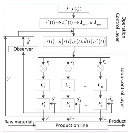
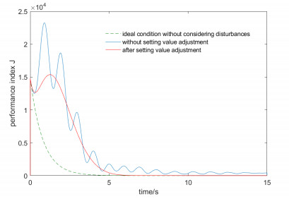
This paper studies a two-layer control strategy for optimal operational control which is prevalent in industrial production. The upper layer determines and adjusts the target set values, while the lower layer makes the loop output track the target value. In the two-layer structure optimal setting control system, the widely used PID controller is used in the bottom layer. Firstly, the parameters of the PID controller are obtained by solving linear matrix inequalities (LMI). Secondly, for industrial processes with nonlinear harmonic disturbances, a disturbance observer is designed to estimate these disturbances. Thirdly, the effects of disturbances or noises are minimized by dynamically adjusting the setting points. This method does not change the structure or parameters of the bottom controller, and thus meets the actual industrial requirements to a certain extent. Finally, in the numerical simulation section, the value of the performance index before set-points adjustment is compared with that after set-points adjustment.
- optimal operational control,
- PID,
- nonlinear,
- disturbance observer,
- set-points reselection
Citation: Liping Yin, Yangyu Zhu, Yangbo Xu, Tao Li. Dynamic optimal operational control for complex systems with nonlinear external loop disturbances[J]. AIMS Mathematics, 2022, 7(9): 16673-16691. doi: 10.3934/math.2022914

Related Papers:

Abstract

This paper studies a two-layer control strategy for optimal operational control which is prevalent in industrial production. The upper layer determines and adjusts the target set values, while the lower layer makes the loop output track the target value. In the two-layer structure optimal setting control system, the widely used PID controller is used in the bottom layer. Firstly, the parameters of the PID controller are obtained by solving linear matrix inequalities (LMI). Secondly, for industrial processes with nonlinear harmonic disturbances, a disturbance observer is designed to estimate these disturbances. Thirdly, the effects of disturbances or noises are minimized by dynamically adjusting the setting points. This method does not change the structure or parameters of the bottom controller, and thus meets the actual industrial requirements to a certain extent. Finally, in the numerical simulation section, the value of the performance index before set-points adjustment is compared with that after set-points adjustment.

References

[1]	A. Wang, P. Zhou, H. Wang, Performance analysis for operational optimal control for complex industrial processes under small loop control errors, In: Proceedings of the 2014 international conference on advanced mechatronic systems, 2014. http://doi.org/10.1109/ICAMechS.2014.6911643
[2]	T. Chai, S. J. Qin, H. Wang, Optimal operational control for complex industrial processes, Annu. Rev. Control, 38 (2014), 81–92. http://doi.org/10.1016/j.arcontrol.2014.03.005 doi: 10.1016/j.arcontrol.2014.03.005
[3]	L. Yin, H. Wang, X. Yan, H. Zhang, Disturbance observer-based dynamic optimal setting control, IET Control Theory A., 12 (2018), 2423–1432. http://doi.org/10.1049/iet-cta.2018.5013 doi: 10.1049/iet-cta.2018.5013
[4]	L. Yin, H. Wang, L. Guo, H. Zhang, Data-driven pareto-de-based intelligent optimal operational control for stochastic processes, IEEE T. Syst. Man Cy. Syst., 51 (2021), 4443–4452. http://doi.org/10.1109/TSMC.2019.2936452 doi: 10.1109/TSMC.2019.2936452
[5]	W. Dai, G. Huang, F. Chu, T. Chai, Configurable platform for optimal-setting control of grinding processes, IEEE Access, 5 (2017), 26722–26733. http://doi.org/10.1109/ACCESS.2017.2774001 doi: 10.1109/ACCESS.2017.2774001
[6]	M. Li, P. Zhou, H. Wang, T. Chai, Nonlinear multiobjective mpc-based optimal operation of a high consistency refining system in papermaking, IEEE T. Syst. Man Cy. Syst., 50 (2017), 1208–1215. http://doi.org/10.1109/TSMC.2017.2748722 doi: 10.1109/TSMC.2017.2748722
[7]	P. Zhou, T. Chai, H. Wang, Intelligent optimal-setting control for grinding circuits of mineral processing process, IEEE T. Autom. Sci. Eng., 6 (2009), 730–743. http://doi.org/10.1109/TASE.2008.2011562 doi: 10.1109/TASE.2008.2011562
[8]	Y. Jiang, J. Fan, T. Chai, J. Li, F. L. Lewis, Data-driven flotation industrial process operational optimal control based on reinforcement learning, IEEE T. Ind. Inform., 14 (2018), 1974–1989. http://doi.org/10.1109/TII.2017.2761852 doi: 10.1109/TII.2017.2761852
[9]	Y. Zhou, Q. Zhang, H. Wang, P. Zhou, T. Chai, Ekf-based enhanced performance controller design for nonlinear stochastic systems, IEEE T. Automat. Contr., 63 (2018), 1155–1162. http://doi.org/10.1109/TAC.2017.2742661 doi: 10.1109/TAC.2017.2742661
[10]	L. Dong, X. Wei, H. Zhang, Anti-disturbance control based on nonlinear disturbance observer for a class of stochastic systems, T. I. Meas. Control, 41 (2019), 1665–1675. http://doi.org/10.1177/0142331218787608 doi: 10.1177/0142331218787608
[11]	S. Xie, Y. Xie, F. Li, C. Yang, W. Gui, Optimal setting and control for iron removal process based on adaptive neural network soft-sensor, IEEE T. Syst. Man Cy. Syst., 50 (2020), 2408–2420. http://doi.org/10.1109/TSMC.2018.2815580 doi: 10.1109/TSMC.2018.2815580
[12]	L. Guo, H. Wang, Stochastic distribution control system design: A convex optimization approach, London: Springer, 2010. http://doi.org/10.1007/978-1-84996-030-4
[13]	Y. Liu, K. Fan, Q. Ouyang, Intelligent traction control method based on model predictive fuzzy pid control and online optimization for permanent magnetic maglev trains, IEEE Access, 9 (2021), 29032–29046. http://doi.org/10.1109/ACCESS.2021.3059443 doi: 10.1109/ACCESS.2021.3059443
[14]	X. Zhou, J. Zhou, C. Yang, W. Gui, Set-point tracking and multi-objective optimization-based pid control for the goethite process, IEEE access, 6 (2018), 36683–36698. http://doi.org/10.1109/ACCESS.2018.2847641 doi: 10.1109/ACCESS.2018.2847641
[15]	C. Liu, Z. Gong, K. L. Teo, J. Sun, L. Caccetta, Robust multi-objective optimal switching control arising in 1, 3-propanediol microbial fed-batch process, Nonlinear Anal. Hybri., 25 (2017), 1–20. http://doi.org/10.1016/j.nahs.2017.01.006 doi: 10.1016/j.nahs.2017.01.006
[16]	C. Liu, Z. Gong, H. W. J. Lee, K. L. Teo, Robust bi-objective optimal control of 1, 3-propanediol microbial batch production process, J. Process Contr., 78 (2019), 170–182. http://doi.org/10.1016/j.jprocont.2018.10.001 doi: 10.1016/j.jprocont.2018.10.001
[17]	B. Li, Y. Wang, K. Zhang, G. R. Duan, Constrained feedback control for spacecraft reorientation with an optimal gain, IEEE T. Aero. Elec. Sys., 57 (2021), 3916–3926. http://doi.org/10.1109/TAES.2021.3082696 doi: 10.1109/TAES.2021.3082696
[18]	J. F. Qiao, Y. Hou, H. G. Han, Optimal control for wastewater treatment process based on an adaptive multi-objective differential evolution algorithm, Neural Comput. Applic., 31 (2019), 2537–2550. http://doi.org/10.1007/s00521-017-3212-4 doi: 10.1007/s00521-017-3212-4
[19]	A. Yan, T. Chai, W. Yu, Z. Xu, Multi-objective evaluation-based hybrid intelligent control optimization for shaft furnace roasting process, Control Eng. Pract., 20 (2012), 857–868. http://doi.org/10.1016/j.conengprac.2012.05.001 doi: 10.1016/j.conengprac.2012.05.001
[20]	Z. Civelek, E. Cam, M. Luy, H. Mamur, Proportional-integral-derivative parameter optimisation of blade pitch controller in wind turbines by a new intelligent genetic algorithm, IET Renew. Power Gen., 10 (2016), 1220–1228. http://doi.org/10.1049/iet-rpg.2016.0029 doi: 10.1049/iet-rpg.2016.0029
[21]	X. Cong, L. Guo, PID control for a class of nonlinear uncertain stochastic systems, In: 2017 IEEE 56th annual conference on decision and control (CDC), 2017. http://doi.org/10.1109/CDC.2017.8263728
[22]	K. Guo, J. Jia, X. Yu, L. Guo, Dual-disturbance observers-based control of uav subject to internal and external disturbances, In: 2019 Chinese automation congress (CAC), 2019. http://doi.org/10.1109/CAC48633.2019.8997330
[23]	C. Zhao, L. Guo, Control of nonlinear uncertain systems by extended pid, IEEE T. Automat. Contr., 66 (2021), 3840–3847. http://doi.org/10.1109/TAC.2020.3030876 doi: 10.1109/TAC.2020.3030876
[24]	C. Zhao, L. Guo, PID control for a class of non-affine uncertain systems, In: 2018 37th Chinese control conference (CCC), 2018. http://doi.org/10.23919/ChiCC.2018.8483587
[25]	S. Yuan, C. Zhao, L. Guo, Decentralized PID control of multi-agent systems with nonlinear uncertain dynamics, In: 2017 36th Chinese control conference (CCC), 2017. http://doi.org/10.23919/ChiCC.2017.8028765
[26]	P. Thampi, G. Raghavendra, Intelligent model for automating PID controller tuning for industrial water level control system, In: 2021 International conference on design innovations for 3Cs compute communicate control (ICDI3C), 2021. http://doi.org/10.1109/ICDI3C53598.2021.00039
[27]	H. Tsukamoto, S. J. Chung, Robust controller design for stochastic nonlinear systems via convex optimization, IEEE T. Automat. Contr., 66 (2021), 4731–4746. http://doi.org/10.1109/TAC.2020.3038402 doi: 10.1109/TAC.2020.3038402
[28]	L. Guo, H. Wang, PID controller design for output pdfs of stochastic systems using linear matrix inequalities, IEEE T. Syst. Man Cy. B, 35 (2005), 65–71. http://doi.org/10.1109/TSMCB.2004.839906 doi: 10.1109/TSMCB.2004.839906
[29]	C. Zhao, L. Guo, PID controller design for second order nonlinear uncertain systems, Sci. China Inf. Sci., 60 (2017), 022201. http://doi.org/10.1007/s11432-016-0879-3 doi: 10.1007/s11432-016-0879-3
[30]	P. Gahinet, A. Nemirovskii, A. J. Laub, M. Chilali, The LMI control toolbox, In: Proceedings of 1994 33rd IEEE conference on decision and control, 1994. http://doi.org/10.1109/CDC.1994.411440
[31]	X. Wei, L. Dong, H. Zhang, X. Hu, J. Han, Adaptive disturbance observer-based control for stochastic systems with multiple heterogeneous disturbances, Int. J. Robust Nonlin., 29 (2019), 5533–5549. http://doi.org/10.1002/rnc.4683 doi: 10.1002/rnc.4683
[32]	X. Wei, S. Sun, Elegant anti-disturbance control for discrete-time stochastic systems with nonlinearity and multiple disturbances, Int. J. Control, 91 (2018), 706–714. http://doi.org/10.1080/00207179.2017.1291996 doi: 10.1080/00207179.2017.1291996
[33]	Z. Ding, Output regulation of uncertain nonlinear systems with nonlinear exosystems, IEEE T. Automat. Contr., 51 (2006), 498–503. http://doi.org/10.1109/TAC.2005.864199 doi: 10.1109/TAC.2005.864199
[34]	M. Lu, J. Huang, A class of nonlinear internal models for global robust output regulation problem, Int. J. Robust Nonlin., 25 (2015), 1831–1843. http://doi.org/10.1002/rnc.3180 doi: 10.1002/rnc.3180
[35]	Y. Xie, S. Xie, Y. Li, C. Yang, W. Gui, Dynamic modeling and optimal control of goethite process based on the rate-controlling step, Control Eng. Pract., 58 (2017), 54–65. http://doi.org/10.1016/j.conengprac.2016.10.001 doi: 10.1016/j.conengprac.2016.10.001

Reader Comments

Your name:*

Email:*
© 2022 the Author(s), licensee AIMS Press. This is an open access article distributed under the terms of the Creative Commons Attribution License (http://creativecommons.org/licenses/by/4.0)