The construction of solutions to $  {}^{C} \mathit{\boldsymbol{{D}}}^{(1/n)} $ type FDEs via reduction to $ \left({}^{C} \mathit{\boldsymbol{{D}}}^{(1/n)}\right)^n $ type FDEs

R. Marcinkevicius; I. Telksniene; T. Telksnys; Z. Navickas; M. Ragulskis; R. Marcinkevicius; I. Telksniene; T. Telksnys; Z. Navickas; M. Ragulskis

doi:10.3934/math.2022905

AIMS Mathematics

2022, Volume 7, Issue 9: 16536-16554. doi: 10.3934/math.2022905

Previous Article Next Article

Research article

The construction of solutions to $ {}^{C} \mathit{\boldsymbol{{D}}}^{(1/n)} $ type FDEs via reduction to $ \left({}^{C} \mathit{\boldsymbol{{D}}}^{(1/n)}\right)^n $ type FDEs

1.
Department of Software Engineering, Kaunas University of Technology, Studentu 50-415, Kaunas LT-51368, Lithuania
2.
Center for Nonlinear Systems, Kaunas University of Technology, Studentu 50-147, Kaunas LT-51368, Lithuania

Received: 26 May 2022 Revised: 05 July 2022 Accepted: 06 July 2022 Published: 08 July 2022
MSC : 34A08, 30B10, 65L99

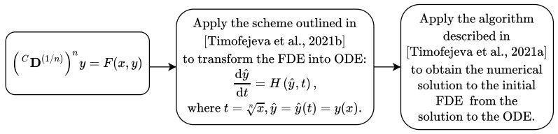
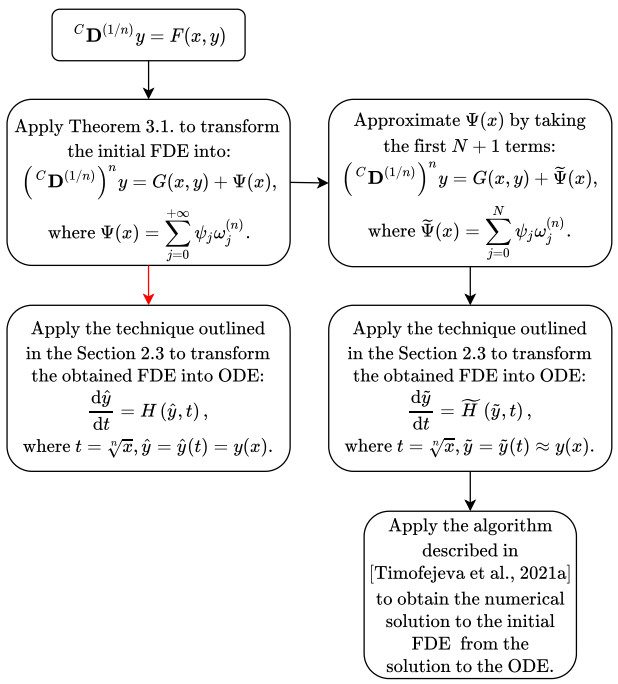
A scheme for the integration of $ \, {}^{C} \mathit{\boldsymbol{{D}}}^{(1/n)} $-type fractional differential equations (FDEs) is presented in this paper. The approach is based on the expansion of solutions to FDEs via fractional power series. It is proven that $ \, {}^{C} \mathit{\boldsymbol{{D}}}^{(1/n)} $-type FDEs can be transformed into equivalent $ \left(\, {}^{C} \mathit{\boldsymbol{{D}}}^{(1/n)}\right)^n $-type FDEs via operator calculus techniques. The efficacy of the scheme is demonstrated by integrating the fractional Riccati differential equation.
- fractional differential equation,
- operator calculus,
- fractional power series expansion
Citation: R. Marcinkevicius, I. Telksniene, T. Telksnys, Z. Navickas, M. Ragulskis. The construction of solutions to $ {}^{C} \mathit{\boldsymbol{{D}}}^{(1/n)} $ type FDEs via reduction to $ \left({}^{C} \mathit{\boldsymbol{{D}}}^{(1/n)}\right)^n $ type FDEs[J]. AIMS Mathematics, 2022, 7(9): 16536-16554. doi: 10.3934/math.2022905

Related Papers:

Abstract

A scheme for the integration of $ \, {}^{C} \mathit{\boldsymbol{{D}}}^{(1/n)} $-type fractional differential equations (FDEs) is presented in this paper. The approach is based on the expansion of solutions to FDEs via fractional power series. It is proven that $ \, {}^{C} \mathit{\boldsymbol{{D}}}^{(1/n)} $-type FDEs can be transformed into equivalent $ \left(\, {}^{C} \mathit{\boldsymbol{{D}}}^{(1/n)}\right)^n $-type FDEs via operator calculus techniques. The efficacy of the scheme is demonstrated by integrating the fractional Riccati differential equation.

References

[1]	R. Alchikh, S. Khuri, Numerical solution of a fractional differential equation arising in optics, Optik, 208 (2020), 163911. https://doi.org/10.1016/j.ijleo.2019.163911 doi: 10.1016/j.ijleo.2019.163911
[2]	M. I. Asjad, W. A. Faridi, K. M. Abualnaja, A. Jhangeer, H. Abu-Zinadah, H. Ahmad, The fractional comparative study of the non-linear directional couplers in non-linear optics, Results Phys., 27 (2021), 104459. https://doi.org/10.1016/j.rinp.2021.104459 doi: 10.1016/j.rinp.2021.104459
[3]	M. S. Asl, M. Javidi, Novel algorithms to estimate nonlinear FDEs: Applied to fractional order nutrient-phytoplankton-zooplankton system, J. Comput. Appl. Math., 339 (2018), 193–207. https://doi.org/10.1016/j.cam.2017.10.030 doi: 10.1016/j.cam.2017.10.030
[4]	D. Baleanu, H. Mohammadi, S. Rezapour, A fractional differential equation model for the COVID-19 transmission by using the Caputo-Fabrizio derivative, Adv. Differ. Equ., 2020 (2020), 1–27. https://doi.org/10.1186/s13662-020-02762-2 doi: 10.1186/s13662-020-02762-2
[5]	A. De Gaetano, S. Sakulrang, A. Borri, D. Pitocco, S. Sungnul, E. J. Moore, Modeling continuous glucose monitoring with fractional differential equations subject to shocks, J. Theor. Biol., 526 (2021), 110776. https://doi.org/10.1016/j.jtbi.2021.110776 doi: 10.1016/j.jtbi.2021.110776
[6]	N. J. Ford, A. C. Simpson, The numerical solution of fractional differential equations: Speed versus accuracy, Numer. Algorithms, 26 (2001), 333–346. https://doi.org/10.1023/A:1016601312158 doi: 10.1023/A:1016601312158
[7]	L. Frunzo, R. Garra, A. Giusti, V. Luongo, Modeling biological systems with an improved fractional gompertz law, Commun. Nonlinear Sci. Numer. Simul., 74 (2019), 260–267. https://doi.org/10.1016/j.cnsns.2019.03.024 doi: 10.1016/j.cnsns.2019.03.024
[8]	R. Garrappa, Numerical solution of fractional differential equations: A survey and a software tutorial, Mathematics, 6 (2018), 16. https://doi.org/10.3390/math6020016 doi: 10.3390/math6020016
[9]	R. Hilfer, Applications of fractional calculus in physics, World Scientific, 2000. https://doi.org/10.1142/3779
[10]	G. Ismail, H. R. Abdl-Rahim, A. Abdel-Aty, R. Kharabsheh, W. Alharbi, M. Abdel-Aty, An analytical solution for fractional oscillator in a resisting medium, Chaos, Solitons Fract., 130 (2020), 109395. https://doi.org/10.1016/j.chaos.2019.109395 doi: 10.1016/j.chaos.2019.109395
[11]	M. D. Johansyah, A. K. Supriatna, E. Rusyaman, J. Saputra, Application of fractional differential equation in economic growth model: A systematic review approach, AIMS Math., 6 (2021), 10266–10280. https://doi.org/10.3934/math.2021594 doi: 10.3934/math.2021594
[12]	R. C. Koeller, Applications of fractional calculus to the theory of viscoelasticity, J. Appl. Mech., 51 (1984), 299–307. https://doi.org/10.1115/1.3167616 doi: 10.1115/1.3167616
[13]	D. Kumar, J. Singh, Fractional calculus in medical and health science, CRC Press, 2020. https://doi.org/10.1201/9780429340567
[14]	C. Li, M. Cai, Theory and numerical approximations of fractional integrals and derivatives, SIAM, 2019. https://doi.org/10.1137/1.9781611975888 doi: 10.1137/1.9781611975888
[15]	Z. Navickas, T. Telksnys, R. Marcinkevicius, M. Ragulskis, Operator-based approach for the construction of analytical soliton solutions to nonlinear fractional-order differential equations, Chaos, Solitons Fract., 104 (2017), 625–634. https://doi.org/10.1016/j.chaos.2017.09.026 doi: 10.1016/j.chaos.2017.09.026
[16]	Z. Navickas, T. Telksnys, I. Timofejeva, R. Marcinkevičius, M. Ragulskis, An operator-based approach for the construction of closed-form solutions to fractional differential equations, Math. Model. Anal., 23 (2018), 665–685. https://doi.org/10.3846/mma.2018.040 doi: 10.3846/mma.2018.040
[17]	J. J. Nieto, Solution of a fractional logistic ordinary differential equation, Appl. Math. Lett., 123 (2022), 107568. https://doi.org/10.1016/j.aml.2021.107568 doi: 10.1016/j.aml.2021.107568
[18]	F. Norouzi, G. M. N'Guérékata, A study of $\psi$-Hilfer fractional differential system with application in financial crisis, Chaos, Solitons Fract.: X, 6 (2021), 100056. https://doi.org/10.1016/j.csfx.2021.100056 doi: 10.1016/j.csfx.2021.100056
[19]	F. W. Olver, D. W. Lozier, R. Boisvert, C. W. Clark, NIST handbook of mathematical functions, Cambridge university press, 2010.
[20]	R. Shah, H. Khan, M. Arif, P. Kumam, Application of Laplace-Adomian decomposition method for the analytical solution of third-order dispersive fractional partial differential equations, Entropy, 21 (2019), 335. https://doi.org/10.3390/e21040335 doi: 10.3390/e21040335
[21]	R. Shah, H. Khan, D. Baleanu, P. Kumam, M. Arif, A novel method for the analytical solution of fractional Zakharov-Kuznetsov equations, Adv. Differ. Equ., 2019 (2019), 1–14. https://doi.org/10.1186/s13662-019-2441-5 doi: 10.1186/s13662-019-2441-5
[22]	R. Shanker Dubey, P. Goswami, Analytical solution of the nonlinear diffusion equation, Eur. Phys. J. Plus, 133 (2018), 1–12. https://doi.org/10.1140/epjp/i2018-12010-6 doi: 10.1140/epjp/i2018-12010-6
[23]	J. Singh, A. Gupta, D. Baleanu, On the analysis of an analytical approach for fractional Caudrey-Dodd-Gibbon equations, Ale. Eng. J., 61 (2022), 5073–5082. https://doi.org/10.1016/j.aej.2021.09.053 doi: 10.1016/j.aej.2021.09.053
[24]	S. Thirumalai, R. Seshadri, S. Yuzbasi, Spectral solutions of fractional differential equations modelling combined drug therapy for hiv infection, Chaos, Solitons Fract., 151 (2021), 111234. https://doi.org/10.1016/j.chaos.2021.111234 doi: 10.1016/j.chaos.2021.111234
[25]	I. Timofejeva, Z. Navickas, T. Telksnys, R. Marcinkevicius, M. Ragulskis, An operator-based scheme for the numerical integration of FDEs, Mathematics, 9 (2021), 1372. https://doi.org/10.3390/math9121372 doi: 10.3390/math9121372
[26]	I. Timofejeva, Z. Navickas, T. Telksnys, R. Marcinkevičius, X. J. Yang, M. Ragulskis, The extension of analytic solutions to FDEs to the negative half-line, AIMS Math., 6 (2021), 3257–3271. https://doi.org/10.3934/math.2021195 doi: 10.3934/math.2021195
[27]	Y. Wei, X. Li, Y. He, Generalisation of tea moisture content models based on vnir spectra subjected to fractional differential treatment, Biosyst. Eng., 205 (2021), 174–186. https://doi.org/10.1016/j.biosystemseng.2021.03.006 doi: 10.1016/j.biosystemseng.2021.03.006
[28]	C. Wen, J. Yang, Complexity evolution of chaotic financial systems based on fractional calculus, Chaos, Solitons Fract., 128 (2019), 242–251. https://doi.org/10.1016/j.chaos.2019.08.005 doi: 10.1016/j.chaos.2019.08.005
[29]	V. F. Zaitsev, A. D. Polyanin, Handbook of exact solutions for ordinary differential equations, CRC Press, 2002.
[30]	J. Zhang, X. Fu, H. Morris, Construction of indicator system of regional economic system impact factors based on fractional differential equations, Chaos, Solitons Fract., 128 (2019), 25–33. https://doi.org/10.1016/j.chaos.2019.07.036 doi: 10.1016/j.chaos.2019.07.036
[31]	Q. Zhou, A. Sonmezoglu, M. Ekici, M. Mirzazadeh, Optical solitons of some fractional differential equations in nonlinear optics, J. Mod. Optics, 64 (2017), 2345–2349. https://doi.org/10.1080/09500340.2017.1357856 doi: 10.1080/09500340.2017.1357856

Reader Comments

Your name:*

Email:*
© 2022 the Author(s), licensee AIMS Press. This is an open access article distributed under the terms of the Creative Commons Attribution License (http://creativecommons.org/licenses/by/4.0)