A spectral collocation method for the coupled system of nonlinear fractional differential equations

Xiaojun Zhou; Yue Dai; Xiaojun Zhou; Yue Dai

doi:10.3934/math.2022314

AIMS Mathematics

2022, Volume 7, Issue 4: 5670-5689. doi: 10.3934/math.2022314

Previous Article Next Article

Research article Special Issues

A spectral collocation method for the coupled system of nonlinear fractional differential equations

Xiaojun Zhou ^,,
Yue Dai

School of Mathematical Sciences, Guizhou Normal University, Guiyang 550025, China

Received: 02 November 2021 Revised: 24 December 2021 Accepted: 28 December 2021 Published: 10 January 2022
MSC : 41A05, 41A10, 41A25, 45D05, 65N35

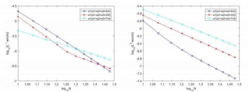
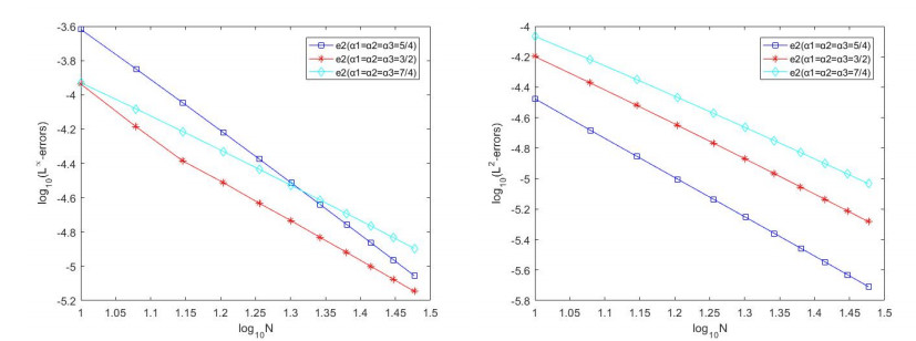
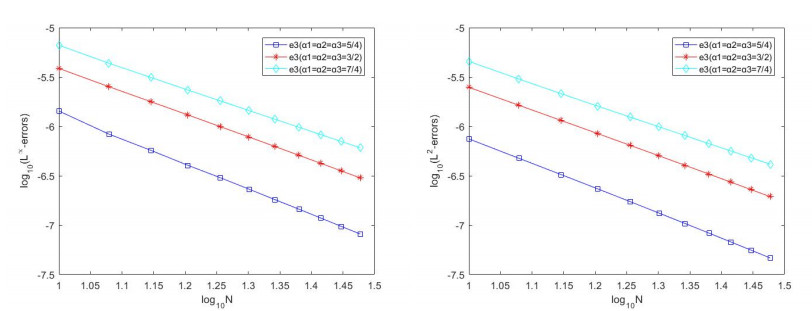
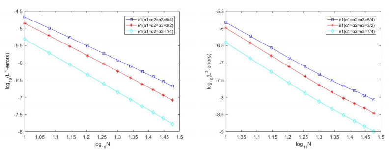
This paper analyzes the coupled system of nonlinear fractional differential equations involving the caputo fractional derivatives of order $ \alpha\in(1, 2) $ on the interval (0, T). Our method of analysis is based on the reduction of the given system to an equivalent system of integral equations, then the resulting equation is discretized by using a spectral method based on the Legendre polynomials. We have constructed a Legendre spectral collocation method for the coupled system of nonlinear fractional differential equations. The error bounds under the $ L^2- $ and $ L^{\infty}- $norms is also provided, then the theoretical result is validated by a number of numerical tests.
- coupled system,
- nonlinear fractional differential equations,
- spectral collocation method,
- caputo fractional derivative,
- error estimates
Citation: Xiaojun Zhou, Yue Dai. A spectral collocation method for the coupled system of nonlinear fractional differential equations[J]. AIMS Mathematics, 2022, 7(4): 5670-5689. doi: 10.3934/math.2022314

Related Papers:

Abstract

This paper analyzes the coupled system of nonlinear fractional differential equations involving the caputo fractional derivatives of order $ \alpha\in(1, 2) $ on the interval (0, T). Our method of analysis is based on the reduction of the given system to an equivalent system of integral equations, then the resulting equation is discretized by using a spectral method based on the Legendre polynomials. We have constructed a Legendre spectral collocation method for the coupled system of nonlinear fractional differential equations. The error bounds under the $ L^2- $ and $ L^{\infty}- $norms is also provided, then the theoretical result is validated by a number of numerical tests.

References

[1]	H. H. Sun, A. A. Abdelwahab, B. Onaral, Linear approximation of transfer function with a pole of fractional power, IEEE T. Automat. Contr., 29 (1984), 441–444. https://doi.org/10.1109/TAC.1984.1103551 doi: 10.1109/TAC.1984.1103551
[2]	A. Oustaloup, La dérivation non entière: Thorie, synthèse et applications, Hermes Science Publications, 1995.
[3]	R. C. Koeller, Applications of fractional calculus to the theory of viscoelasticity, J. Appl. Mech., 51 (1984), 299–307. https://doi.org/10.1115/1.3167616 doi: 10.1115/1.3167616
[4]	R. L. Bagley, R. A. Calico, Fractional order state equations for the control of viscoelasticallydamped structures, J. Guid. Control Dynam., 14 (1991), 304–311. https://doi.org/10.2514/3.20641 doi: 10.2514/3.20641
[5]	F. Amblard, A. C. Maggs, B. Yurke, A. N. Pargellis, S. Leibler, Subdiffusion and anomalous local viscoelasticity in actin networks, Phys. Rev. Lett., 77 (1996), 4470–4473. https://doi.org/10.1103/PhysRevLett.77.4470 doi: 10.1103/PhysRevLett.77.4470
[6]	B. Mandelbrot, Some noises with 1/f spectrum, a bridge between direct current and white noise, IEEE T. Inf. Theory., 13 (1967), 289–298. https://doi.org/10.1109/TIT.1967.1053992 doi: 10.1109/TIT.1967.1053992
[7]	G. E. Carlson, C, Halijak, Approximation of fractional capacitors by a regular newton process, IEEE T. Circuit Theory, 11 (1964), 210–213. https://doi.org/10.1109/TCT.1964.1082270 doi: 10.1109/TCT.1964.1082270
[8]	J. P. Bouchaud, A. Georges, Anomalous diffusion in disordered media: Statistical mechanisms, models and physical applications, Phys. Rep., 195 (1990), 127–293. https://doi.org/10.1016/0370-1573(90)90099-N doi: 10.1016/0370-1573(90)90099-N
[9]	I. Goychuk, E. Heinsalu, M. Patriarca, G. Schmid, P. Hanggi, Current and universal scaling in anomalous transport, Phys. Rev. E, 73 (2006), 020101. https://doi.org/10.1103/PhysRevE.73.020101 doi: 10.1103/PhysRevE.73.020101
[10]	R. Klages, G. Radons, I. M. Sokolov, Anomalous transport: Foundations and applications, Wiley-VCH Verlag, 2008. https://doi.org/10.1002/9783527622979
[11]	K. M. Saad, M. Alqhtani, Numerical simulation of the fractal-fractional reaction diffusion equations with general nonlinear, AIMS Math., 6 (2021), 3788–3804. https://doi.org/10.3934/math.2021225 doi: 10.3934/math.2021225
[12]	H. M. Srivastava, K. M. Saad, M. Khader, An efficient spectral collocation method for the dynamic simulation of the fractional epidemiological model of the Ebola virus, Chaos Solitons Fractals, 140 (2020), 110174. https://doi.org/10.1016/j.chaos.2020.110174 doi: 10.1016/j.chaos.2020.110174
[13]	H. Amann, Parabolic evolution equations and nonlinear boundary conditions, J. Differ. Equations, 72 (1988), 201–269. https://doi.org/10.1016/0022-0396(88)90156-8 doi: 10.1016/0022-0396(88)90156-8
[14]	C. V. Pao, Finite difference reaction diffusion systems with coupled boundary conditions and time delays, J. Math. Anal. Appl., 272 (2002), 407–434. https://doi.org/10.1016/S0022-247X(02)00145-2 doi: 10.1016/S0022-247X(02)00145-2
[15]	S. Wang, Doubly nonlinear degenerate parabolic systems with coupled nonlinear boundary conditions, J. Differ. Equations, 182 (2002), 431–469. https://doi.org/10.1006/jdeq.2001.4101 doi: 10.1006/jdeq.2001.4101
[16]	X. W. Su, Boundary value problem for a coupled system of nonlinear fractional differential equations, Appl. Math. Lett., 22 (2009), 64–69. https://doi.org/10.1016/j.aml.2008.03.001 doi: 10.1016/j.aml.2008.03.001
[17]	M. J. Li, Y. L. Liu, Existence and uniqueness of positive solutions for a coupled system of nonlinear fractional differential equations, Open J. Appl. Sci., 3 (2013), 53–61. https://doi.org/10.4236/ojapps.2013.31B1011 doi: 10.4236/ojapps.2013.31B1011
[18]	Y. Wang, S. Liang, Q. Wang, Existence results for fractional differential equations with integral and multi-point boundary conditions, Bound. Value Probl., 2018 (2018), 4. https://doi.org/10.1186/s13661-017-0924-4 doi: 10.1186/s13661-017-0924-4
[19]	B. Ahmad, S. Hamdan, A. Alsaedi, S. K. Ntouyas, A study of a nonlinear coupled system of three fractional differential equations with nonlocal coupled boundary conditions, Adv. Differ. Equ., 2021 (2021), 1–21. https://doi.org/10.1186/s13662-021-03440-7 doi: 10.1186/s13662-021-03440-7
[20]	J. H. Wang, H. J. Xiang, Z. G. Liu, Positive solution to nonzero boundary values problem for a coupled system of nonlinear fractional differential equations, Int. J. Differ. Equ., 2010 (2010), 186928. https://doi.org/10.1155/2010/186928 doi: 10.1155/2010/186928
[21]	W. G. Yang, Positive solutions for a coupled system of nonlinear fractional differential equations with integral boundary conditions, Comput. Math. Appl., 63 (2012), 288–297. https://doi.org/10.1016/j.camwa.2011.11.021 doi: 10.1016/j.camwa.2011.11.021
[22]	Y. Wang, L. S. Liu, Y. H. Wu, Positive solutions for a class of higher-order singular semipositone fractional differential systems with coupled integral boundary conditions and parameters, Adv. Differ. Equ., 2014 (2014), 268. https://doi.org/10.1186/1687-1847-2014-268 doi: 10.1186/1687-1847-2014-268
[23]	Z. Odibat, S. Momani, Modified homotopy perturbation method: Application to quadratic riccati differential equation of fractional order, Chaos Solitons Fractals, 36 (2008), 167–174. https://doi.org/10.1016/j.chaos.2006.06.041 doi: 10.1016/j.chaos.2006.06.041
[24]	H. Jafari, V. Daftardar-Gejji, Solving a system of nonlinear fractional differential equations using adomian decomposition, J. Comput. Appl. Math., 196 (2006), 644–651. https://doi.org/10.1016/j.cam.2005.10.017 doi: 10.1016/j.cam.2005.10.017
[25]	S. Momani, Z. Odibat, Numerical approach to differential equations of fractional order, J. Comput. Appl. Math., 207 (2007), 96–110. https://doi.org/10.1016/j.cam.2006.07.015 doi: 10.1016/j.cam.2006.07.015
[26]	X. J. Zhou, C. J. Xu, Numerical solution of the coupled system of nonlinear fractional ordinary differential equations, Adv. Appl. Math. Mech., 9 (2017), 574–595. https://doi.org/10.4208/aamm.2015.m1054 doi: 10.4208/aamm.2015.m1054
[27]	C. L. Wang, Z. Q. Wang, L. L. Wang, A spectral collocation method for nonlinear fractional boundary value problems with a caputo derivative, J. Sci. Comput., 76 (2018), 166–188. https://doi.org/10.1007/s10915-017-0616-3 doi: 10.1007/s10915-017-0616-3
[28]	A. Kilbas, H. M. Srivastava, J. J. Trujillo, Theory and applications of fractional differential equations, Elsevier, 2006.
[29]	J. Shen, T. Tang, Z. H. Teng, Spectral and high-order methods with applications, 2006.

Reader Comments

Your name:*

Email:*
© 2022 the Author(s), licensee AIMS Press. This is an open access article distributed under the terms of the Creative Commons Attribution License (http://creativecommons.org/licenses/by/4.0)