On the study of solutions of Bogoyavlenskii equation via improved $ G'/G^2 $ method and simplified $ \tan(\phi(\xi)/2) $ method

Guowei Zhang; Jianming Qi; Qinghao Zhu; Guowei Zhang; Jianming Qi; Qinghao Zhu

doi:10.3934/math.20221078

AIMS Mathematics

2022, Volume 7, Issue 11: 19649-19663. doi: 10.3934/math.20221078

Previous Article Next Article

Research article

On the study of solutions of Bogoyavlenskii equation via improved $ G'/G^2 $ method and simplified $ \tan(\phi(\xi)/2) $ method

1.
School of Mathematics and Statistics, Anyang Normal University, Anyang, Henan, 455000, China
2.
School of Business, Shanghai Dianji University, Shanghai, 201306, China

Received: 21 June 2022 Revised: 27 August 2022 Accepted: 28 August 2022 Published: 06 September 2022
MSC : 34A05, 35C07, 35G20

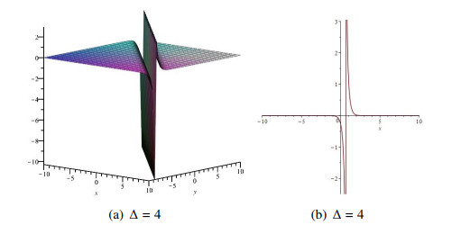
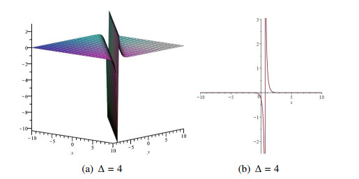
The Bogoyavlenskii equation is used to describe some kinds of waves on the sea surface and discussed by many researchers. Recently, the $ G'/G^2 $ method and simplified $ \tan(\frac{\phi(\xi)}{2}) $ method are introduced to find novel solutions to differential equations. To the best of our knowledge, the Bogoyavlenskii equation has not been investigated by these two methods. In this article, we applied these two methods to the Bogoyavlenskii equation in order to obtain the novel exact traveling wave solutions. Consequently, we found that some new rational functions, trigonometric functions, and hyperbolic functions can be the traveling wave solutions of this equation. Some of these solutions we obtained have not been reported in the former literature. Through comparison, we see that the two methods are more effective than the previous methods for this equation. In order to make these solutions more obvious, we draw some 3D and 2D plots of them.
- soliton,
- traveling wave solution,
- Bogoyavlenskii equation
Citation: Guowei Zhang, Jianming Qi, Qinghao Zhu. On the study of solutions of Bogoyavlenskii equation via improved $ G'/G^2 $ method and simplified $ \tan(\phi(\xi)/2) $ method[J]. AIMS Mathematics, 2022, 7(11): 19649-19663. doi: 10.3934/math.20221078

Related Papers:

Abstract

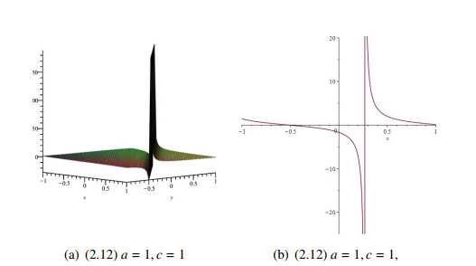
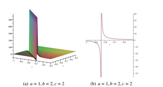
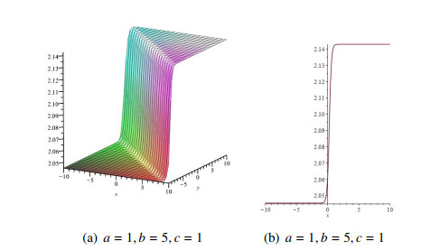
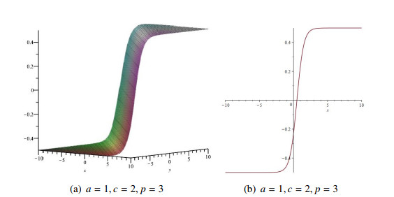
The Bogoyavlenskii equation is used to describe some kinds of waves on the sea surface and discussed by many researchers. Recently, the $ G'/G^2 $ method and simplified $ \tan(\frac{\phi(\xi)}{2}) $ method are introduced to find novel solutions to differential equations. To the best of our knowledge, the Bogoyavlenskii equation has not been investigated by these two methods. In this article, we applied these two methods to the Bogoyavlenskii equation in order to obtain the novel exact traveling wave solutions. Consequently, we found that some new rational functions, trigonometric functions, and hyperbolic functions can be the traveling wave solutions of this equation. Some of these solutions we obtained have not been reported in the former literature. Through comparison, we see that the two methods are more effective than the previous methods for this equation. In order to make these solutions more obvious, we draw some 3D and 2D plots of them.

References

[1]	J. Weiss, Bäcklund transformation and the Painlevé property, J. Math. Phys., 27 (1986), 1293–1305. https://doi.org/10.1063/1.527134 doi: 10.1063/1.527134
[2]	M. L. Wang, Y. M. Wang, Y. B. Zhou, An auto-Backlund transformation and exact solutions to a generalized KdV equation with variable coefficients and their applications, Phys. Lett. A, 303 (2002), 45–51. https://doi.org/10.1016/S0375-9601(02)00975-1 doi: 10.1016/S0375-9601(02)00975-1
[3]	D. G. Zhang, Integrability of fermionic extensions of the Burgers equation, Phys. Lett. A, 223 (1996), 436–438. https://doi.org/10.1016/S0375-9601(96)00773-6 doi: 10.1016/S0375-9601(96)00773-6
[4]	Y. Y. Gu, Analytical solutions to the Caudrey-Dodd-Gibbon-Sawada-Kotera equation via symbol calculation approach, J. Funct. Space., 2020 (2020), 5042724. https://doi.org/10.1155/2020/5042724 doi: 10.1155/2020/5042724
[5]	E. Zayed, Y. A. Amer, A. H. Arnous, Functional variable method and its applications for finding exact solutions of nonlinear PDEs in mathematical physics, Sci. Res. Essays, 8 (2013), 2068–2074. https://doi.org/10.5897/SRE2013.5725 doi: 10.5897/SRE2013.5725
[6]	M. N. Alam, M. A. Akbar, Exact traveling wave solutions of the KP-BBM equation by using the new approach of generalized (G'/G)-expansion method, SpringerPlus, 2 (2013), 617. https://doi.org/10.1186/2193-1801-2-617 doi: 10.1186/2193-1801-2-617
[7]	J. Satsuma, Hirota bilinear method for nonlinear evolution equations, In: Direct and tnverse methods in nonlinear evolution equations, Berlin: Springer, 2003. https://doi.org/10.1007/978-3-540-39808-0_4
[8]	J. Weiss, M. Tabor, G. Carnevale, The Painlevé property for partial differential equations, J. Math. Phys., 24 (1983), 522. https://doi.org/10.1063/1.525721 doi: 10.1063/1.525721
[9]	W. Hereman, M. Takaoka, Solitary wave solutions of nonlinear evolution and wave equations using a direct method and MACSYMA, J. Phys. A Math. Gen., 23 (1990), 4805. https://doi.org/10.1088/0305-4470/23/21/021 doi: 10.1088/0305-4470/23/21/021
[10]	S. T. Mohyud-Din, A. Irshad, Solitary wave solutions of some nonlinear PDEs arising in electronics, Opt. Quant. Electron., 49 (2017), 130. https://doi.org/10.1007/s11082-017-0974-y doi: 10.1007/s11082-017-0974-y
[11]	A. Patel, V. Kumar, Dark and kink soliton solutions of the generalized ZK–BBM equation by iterative scheme, Chinese J. Phys., 56 (2018), 819–829. https://doi.org/10.1016/j.cjph.2018.03.012 doi: 10.1016/j.cjph.2018.03.012
[12]	N. H. Aljahdaly, A. R. Seadawy, W. A. Albarakati, Applications of dispersive analytical wave solutions of nonlinear seventh order Lax and Kaup-Kupershmidt dynamical wave equations, Results Phys., 14 (2019), 102372. https://doi.org/10.1016/j.rinp.2019.102372 doi: 10.1016/j.rinp.2019.102372
[13]	N. H. Aljahdaly, A. R. Seadawy, W. A. Albarakati, Analytical wave solution for the generalized nonlinear seventh-order KdV dynamical equations arising in shallow water waves, Mod. Phys. Lett. B, 34 (2020), 2050279. https://doi.org/10.1142/S0217984920502796 doi: 10.1142/S0217984920502796
[14]	M. I. Tarikul, M. A. Akbar, J. F. Gómez-Aguilar, E. Bonyahd, G. Fernandez-Anaya, Assorted soliton structures of solutions for fractional nonlinear Schrodinger types evolution equations, J. Ocean Eng. Sci., 2021. https://doi.org/10.1016/j.joes.2021.10.006
[15]	M. M. A. Khater, A. Jhangeer, H. Rezazadeh, L. Akinyemi, M. A. Akbar, M. Inc, Propagation of new dynamics of longitudinal bud equation among a magneto-electro-elastic round rod, Mod. Phys. Lett. B, 35 (2021), 2150381. https://doi.org/10.1142/S0217984921503814 doi: 10.1142/S0217984921503814
[16]	K. S. Nisar, K. K. Ali, M. Inc, M. S. Mehanna, H. Rezazadeh, L. Akinyemi, New solutions for the generalized resonant nonlinear Schrödinger equation, Results Phys., 33 (2022), 105153. https://doi.org/10.1016/j.rinp.2021.105153 doi: 10.1016/j.rinp.2021.105153
[17]	L. Akinyemi, M. Senol, E. Az-Zo'bi, P. Veeresha, U. Akpan, Novel soliton solutions of four sets of generalized (2+1)-dimensional Boussinesq-Kadomtsev-Petviashvili-like equations, Mod. Phys. Lett. B, 36 (2022), 2150530 https://doi.org/10.1142/S0217984921505308 doi: 10.1142/S0217984921505308
[18]	M. S. Osman, H. I. Abdel-Gawad, M. A. El Mahdy, Two-layer-atmospheric blocking in a medium with high nonlinearity and lateral dispersion, Results Phys., 8 (2018), 1054–1060. https://doi.org/10.1016/j.rinp.2018.01.040 doi: 10.1016/j.rinp.2018.01.040
[19]	A. A. J. Gaber, Solitary and periodic wave solutions of (2+1)-dimensions of dispersive long wave equations on shallow water, J. Ocean Eng. Sci., 6 (2021), 292–298. https://doi.org/10.1016/j.joes.2021.02.002 doi: 10.1016/j.joes.2021.02.002
[20]	S. F. Tian, J. M. Tu, T. T. Zhang, Y. R. Chen, Integrable discretizations and soliton solutions of an Eckhaus-Kundu equation, Appl. Math. Lett., 122 (2021), 107507 https://doi.org/10.1016/j.aml.2021.107507 doi: 10.1016/j.aml.2021.107507
[21]	S. F. Tian, M. J. Xu, T. T. Zhang, A symmetry-preserving difference scheme and analytical solutions of a generalized higher-order beam equation, Proc. R. Soc. A, 477 (2021), 20210455. https://doi.org/10.1098/rspa.2021.0455 doi: 10.1098/rspa.2021.0455
[22]	S. F. Tian, Lie symmetry analysis, conservation laws and solitary wave solutions to a fourth-order nonlinear generalized Boussinesq water wave equation, Appl. Math. Lett., 100 (2020), 106056. https://doi.org/10.1016/j.aml.2019.106056 doi: 10.1016/j.aml.2019.106056
[23]	M. Adel, D. Baleanu, U. Sadiya, M. A. Arefin, M. Hafiz Uddin, Mahjoub A. Elamin, et al., Inelastic soliton wave solutions with different geometrical structures to fractional order nonlinear evolution equations, Results Phys., 38 (2022), 105661. https://doi.org/10.1016/j.rinp.2022.105661 doi: 10.1016/j.rinp.2022.105661
[24]	A. Zafar, M. Raheel, M. Q. Zafar, K. S. Nisar, M. S. Osman, R. N. Mohamed, et al., Dynamics of different nonlinearities to the perturbed nonlinear schrödinger equation via solitary wave solutions with numerical simulation, Fractal Fract., 5 (2021), 213. https://doi.org/10.3390/fractalfract5040213 doi: 10.3390/fractalfract5040213
[25]	M. Mirzazadeh, A. Akbulut, F. Tascan, L. Akinyemi, A novel integration approach to study the perturbed Biswas-Milovic equation with Kudryashov's law of refractive index, Optik, 252 (2022), 168529. https://doi.org/10.1016/j.ijleo.2021.168529 doi: 10.1016/j.ijleo.2021.168529
[26]	O. I. Bogoyavlenskii, Breaking solitons in 2+1-dimensional integrable equations, Russ. Math. Surv., 45 (1990), 1. https://doi.org/10.1070/RM1990v045n04ABEH002377 doi: 10.1070/RM1990v045n04ABEH002377
[27]	N. Kudryashov, A. Pickering, Rational solutions for the Schwarzian integrable hierarchies, J. Phys. A Math. Gen., 31 (1998), 9505. https://doi.org/10.1088/0305-4470/31/47/011 doi: 10.1088/0305-4470/31/47/011
[28]	P. A. Clarkson, P. R. Gordoa, A. Pickering, Multicomponent equations associated to non-isospectral scattering problems, Inverse Probl., 13 (1997), 1463. https://doi.org/10.1088/0266-5611/13/6/004 doi: 10.1088/0266-5611/13/6/004
[29]	P. G. Estevez, J. Prada, A generalization of the sine-Gordon equation to (2+1)-dimensions, J. Nonlinear Math. Phy., 11 (2004), 164–179. https://doi.org/10.2991/jnmp.2004.11.2.3 doi: 10.2991/jnmp.2004.11.2.3
[30]	Y. Z. Peng, S. Ming, On exact solutions of the bogoyavlenskii equation, Pramana, 67 (2006), 449–456. https://doi.org/10.1007/s12043-006-0005-1 doi: 10.1007/s12043-006-0005-1
[31]	E. Zahran, M. A. Khater, Modified extended tanh-function method and its applications to the Bogoyavlenskii equation, Appl. Math. Model., 40 (2016), 1769–1775. https://doi.org/10.1016/j.apm.2015.08.018 doi: 10.1016/j.apm.2015.08.018
[32]	A. Malik, F. Chand, H. Kumar, S. C. Mishra, Exact solutions of the Bogoyavlenskii equation using the multiple ($G'/G$)-expansion method, Comput. Math. Appl., 64 (2012), 2850–2859. https://doi.org/10.1016/j.camwa.2012.04.018 doi: 10.1016/j.camwa.2012.04.018
[33]	J. Yu, Y. Sun, Modified method of simplest equation and its applications to the Bogoyavlenskii equation, Comput. Math. Appl., 72 (2016), 1943–1955. https://doi.org/10.1016/j.camwa.2016.08.002 doi: 10.1016/j.camwa.2016.08.002
[34]	A. Yokus, H. Durur, H. Ahmad, P. Thounthong, Y. F. Zhang, Construction of exact traveling wave solutions of the Bogoyavlenskii equation by $(G'/G, 1/G)$-expansion and $(1/G')$-expansion techniques, Results Phys., 19 (2020), 103409. https://doi.org/10.1016/j.rinp.2020.103409 doi: 10.1016/j.rinp.2020.103409
[35]	N. H. Aljahdaly, Aly R. Seadawy, Wafaa A. Albarakati, Applications of dispersive analytical wave solutions of nonlinear seventh order Lax and Kaup-Kupershmidt dynamical wave equations, Results Phys., 14 (2019), 102372. https://doi.org/10.1016/j.rinp.2019.102372 doi: 10.1016/j.rinp.2019.102372
[36]	S. Behera, N. H. Aljahdaly, J. P. S. Virdi, On the modified ($G'/G^2$)-expansion method for finding some analytical solutions of the traveling waves, J. Ocean Eng. Sci., 7 (2022), 313–320. https://doi.org/10.1016/j.joes.2021.08.013 doi: 10.1016/j.joes.2021.08.013
[37]	H. Chen, Q. Zhu, J. Qi, Further results about the exact solutions of conformable space-time fractional Boussinesq equation (FBE) and breaking soliton (Calogero) equation, Results Phys., 37 (2022), 105428. https://doi.org/10.1016/j.rinp.2022.105428 doi: 10.1016/j.rinp.2022.105428
[38]	J. Manafian, M. Lakestani, Application of $\tan(\phi/2)$-expansion method for solving the Biswas-Milovic equation for Kerr law nonlinearity, Optik, 127 (2016), 2040–2054. https://doi.org/10.1016/j.ijleo.2015.11.078 doi: 10.1016/j.ijleo.2015.11.078
[39]	J. Manafian, Optical soliton solutions for Schrödinger type nonlinear evolution equations by the $\tan(\phi/2)$-expansion method, Optik, 127 (2016), 4222–4245. https://doi.org/10.1016/j.ijleo.2016.01.078 doi: 10.1016/j.ijleo.2016.01.078
[40]	H. Liu, T. Zhang, A note on the improved $\tan(\phi/2)$-expansion method, Optik, 131 (2017), 273–278. https://doi.org/10.1016/j.ijleo.2016.11.029 doi: 10.1016/j.ijleo.2016.11.029
[41]	H. C. Yaslan, A. Girgin, SITEM for the conformable space-time fractional Boussinesq and (2+1)-dimensional breaking solition equations, J. Ocean Eng. Sci., 6 (2021), 228–236. https://doi.org/10.1016/j.joes.2020.11.010 doi: 10.1016/j.joes.2020.11.010

Reader Comments

Your name:*

Email:*
© 2022 the Author(s), licensee AIMS Press. This is an open access article distributed under the terms of the Creative Commons Attribution License (http://creativecommons.org/licenses/by/4.0)