A new approach to persistence and periodicity of logistic systems with jumps

Kegang Zhao; Kegang Zhao

doi:10.3934/math.2021709

AIMS Mathematics

2021, Volume 6, Issue 11: 12245-12259. doi: 10.3934/math.2021709

Previous Article Next Article

Research article

A new approach to persistence and periodicity of logistic systems with jumps

Kegang Zhao ^,

School of physical education, Shandong Normal University, Jinan, 250014, China

Received: 02 July 2021 Accepted: 15 August 2021 Published: 25 August 2021
MSC : 34A37, 34D20

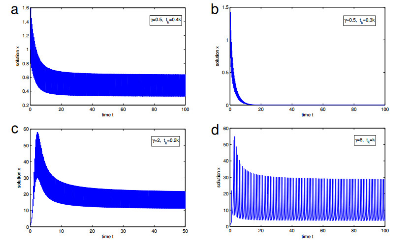
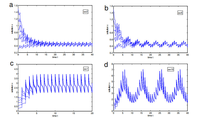
This paper considers a class of logistic type differential system with jumps. Based on discontinuous control theory, a new approach is developed to guarantee the persistence and existence of a unique globally attractive positive periodic solution. The development results of this paper emphasize the effects of jumps on system, which are different from the existing ones in the literature. Two examples and their simulations are given to illustrate the effectiveness of the proposed results.
- logistic differential system,
- persistence,
- periodicity,
- globally attractive,
- jumps
Citation: Kegang Zhao. A new approach to persistence and periodicity of logistic systems with jumps[J]. AIMS Mathematics, 2021, 6(11): 12245-12259. doi: 10.3934/math.2021709

Related Papers:

Abstract

This paper considers a class of logistic type differential system with jumps. Based on discontinuous control theory, a new approach is developed to guarantee the persistence and existence of a unique globally attractive positive periodic solution. The development results of this paper emphasize the effects of jumps on system, which are different from the existing ones in the literature. Two examples and their simulations are given to illustrate the effectiveness of the proposed results.

References

[1]	K. Gopalsamy, Stability and oscillations in delay differential equations of population dynamics, Springer Science & Business Media, 1992.
[2]	G. Consolini, M. Materassi, A stretched logistic equation for pandemic spreading, Chaos Soliton. Fract., 140 (2020), 110113. doi: 10.1016/j.chaos.2020.110113
[3]	C. Burgos, J. C. Cortés, E. López-Navarro, R. J. Villanueva, Probabilistic analysis of linear-quadratic logistic-type models with hybrid uncertainties via probability density functions, AIMS Mathematics, 6 (2021), 4938–4957. doi: 10.3934/math.2021290
[4]	G. Ascione, Abstract Cauchy problems for generalized fractional calculus, Nonlinear Anal., 209 (2021), 112339. doi: 10.1016/j.na.2021.112339
[5]	W. Cintra, C. Morales-Rodrigo, A. Suárez, Refuge versus dispersion in the logistic equation, J. Differ. Equations, 262 (2017), 5606–5634. doi: 10.1016/j.jde.2017.02.012
[6]	I. Area, J. Losada, J. J. Nieto, A note on the fractional logistic equation, Physica A, 444 (2016), 182–187. doi: 10.1016/j.physa.2015.10.037
[7]	M. Delgado, M. Molina-Becerra, A. Suárez, A logistic type equation in $\mathbb{R}^N$ with a nonlocal reaction term via bifurcation method, J. Math. Anal. Appl., 493 (2021), 124532. doi: 10.1016/j.jmaa.2020.124532
[8]	M. Liu, K. Wang, On a stochastic logistic equation with impulsive perturbations, Comput. Math. Appl., 63 (2012), 871–886.
[9]	P. Korman, On separated solutions of logistic population equation with harvesting, J. Math. Anal. Appl., 455 (2017), 2024–2029. doi: 10.1016/j.jmaa.2017.06.029
[10]	M. D'Ovidio, Non-local logistic equations from the probability viewpoint, arXiv: 2105.00779.
[11]	M. D'Ovidio, Solutions of fractional logistic equations by Euler's numbers, Physica A, 506 (2018), 1081–1092. doi: 10.1016/j.physa.2018.05.030
[12]	C. Holling, Some characteristics of simple types of predation and parasitism, Can. Entomol., 91 (1959), 385–398. doi: 10.4039/Ent91385-7
[13]	A. Hasting, Population biology: Concepts and models, New York: Springer, 1997.
[14]	M. Kot, Elements of mathematical ecology, Cambridge University Press, 2001.
[15]	F. Brauer, C. Castilo-Chavez, Mathematical models in population biology and epidemiology, New York: Springer, 2001.
[16]	X. Yang, X. Li, Q. Xi, P. Duan, Review of stability and stabilization for impulsive delayed systems, Math. Biosci. Eng., 15 (2018), 1495–1515. doi: 10.3934/mbe.2018069
[17]	D. Bainov, P. Simeonov, Impulsive differential equations: Periodic solutions and applications, CRC Press, 1993.
[18]	Z. Li, X. Shu, F. Xu, The existence of upper and lower solutions to second order random impulsive differential equation with boundary value problem, AIMS Mathematics, 5 (2020), 6189–6210. doi: 10.3934/math.2020398
[19]	X. Li, J. Shen, R. Rakkiyappan, Persistent impulsive effects on stability of functional differential equations with finite or infinite delay, Appl. Math. Comput., 329 (2018), 14–22.
[20]	G. Ballinger, X. Liu, Permanence of population growth models with impulsive effects, Math. Comput. Model., 26 (1997), 59–72.
[21]	I. Stamova, G. T. Stamov, Applied impulsive mathematical models, Switzerland: Springer, 2016.
[22]	Z. Teng, L. Nie, X. Fang, The periodic solutions for general periodic impulsive population systems of functional differential equations and its applications, Comput. Math. Appl., 61 (2011), 2690–2703. doi: 10.1016/j.camwa.2011.03.023
[23]	D. Yang, X. Li, Z. Liu, J. Cao, Persistence of nonautonomous logistic system with time-varying delays and impulsive perturbations, Nonlinear Anal. Model., 25 (2020), 564–579.
[24]	A. N. Churilov, Orbital stability of periodic solutions of an impulsive system with a linear continuous-time part, AIMS Mathematics, 5 (2020), 96–110. doi: 10.3934/math.2020007
[25]	G. Stamov, E. Gospodinova, I. Stamova, Practical exponential stability with respect to h-manifolds of discontinuous delayed Cohen-Grossberg neural networks with variable impulsive perturbations, Math. Model. Control, 1 (2021), 26–34. doi: 10.3934/mmc.2021003
[26]	P. Li, X. Li, J. Cao, Input-to-state stability of nonlinear switched systems via Lyapunov method involving indefinite derivative, Complexity, 2018 (2018), 8701219.
[27]	M. Liu, S. Li, X. Li, L. Jin, C. Yi, Intelligent controllers for multirobot competitive and dynamic tracking, Complexity, 2018 (2018), 4573631.
[28]	T. Wei, X. Xie, X. Li, Input-to-state stability of delayed reaction-diffusion neural networks with multiple impulses, AIMS Mathematics, 6 (2021), 5786–5800. doi: 10.3934/math.2021342
[29]	X. Zhang, Z. Shuai, K. Wang, Optimal impulsive harvesting policy for single population, Nonlinear Anal. Real, 4 (2003), 639–651. doi: 10.1016/S1468-1218(02)00084-6
[30]	V. Lakshmikantham, D. D. Bainov, P. S. Simeonov, Theory of impulsive differential equations, World Scientific, 1989.

Reader Comments

Your name:*

Email:*
© 2021 the Author(s), licensee AIMS Press. This is an open access article distributed under the terms of the Creative Commons Attribution License (http://creativecommons.org/licenses/by/4.0)