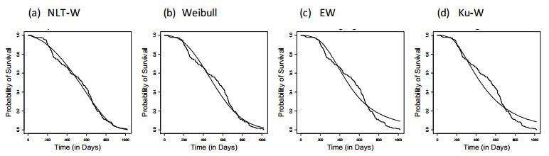
In data science, it is frequent that new and sophisticated computational methods and tools are used to build predictive models to perform time to event data analysis. Such predictive models based on previously collected data from patients can support decision-making and prediction for the clinical data. Hence, this paper introduced a novel superior distribution, namely a new lifetime Weibull (NLT-W) distribution, using an efficient method to generate new distributions called the T-X method for generating new distributions. Parameter estimation has been done through maximum likelihood estimation (MLE) to show the significance of this proposed model over other competitive models. Comparison to two-parameter Weibull, Exponentiated Weibull (EW), and the and the Kumaraswamy Weibull (Ku-W) indicates that the proposed model could preform better to model various types of survival.
Citation: Heba S. Mohammed, Zubair Ahmad, Alanazi Talal Abdulrahman, Saima K. Khosa, E. H. Hafez, M. M. Abd El-Raouf, Marwa M. Mohie El-Din. Statistical modelling for Bladder cancer disease using the NLT-W distribution[J]. AIMS Mathematics, 2021, 6(9): 9262-9276. doi: 10.3934/math.2021538
In data science, it is frequent that new and sophisticated computational methods and tools are used to build predictive models to perform time to event data analysis. Such predictive models based on previously collected data from patients can support decision-making and prediction for the clinical data. Hence, this paper introduced a novel superior distribution, namely a new lifetime Weibull (NLT-W) distribution, using an efficient method to generate new distributions called the T-X method for generating new distributions. Parameter estimation has been done through maximum likelihood estimation (MLE) to show the significance of this proposed model over other competitive models. Comparison to two-parameter Weibull, Exponentiated Weibull (EW), and the and the Kumaraswamy Weibull (Ku-W) indicates that the proposed model could preform better to model various types of survival.

| [1] | P. M. Gurung, A. Veerakumarasivam, M. Williamson, N. Counsell, J. Douglas, W. S. Tan, et al., Loss of expression of the tumour suppressor gene AIMP3 predicts survival following radiotherapy in muscle‐invasive bladder cancer, Int. J. Cancer, 136 (2015), 709–720. |
| [2] |
M. Riester, J. M. Taylor, A. Feifer, T. Koppie, J. E. Rosenberg, R. J. Downey, et al., Combination of a novel gene expression signature with a clinical nomogram improves the prediction of survival in high-risk bladder cancer, Clin. Cancer Res., 18 (2012), 1323–1333. doi: 10.1158/1078-0432.CCR-11-2271

|
| [3] |
F. Bray, J. Ferlay, I. Soerjomataram, R. L. Siegel, L. Torre, A. Jemal, Global cancer statistics 2018: GLOBOCAN estimates of incidence and mortality worldwide for 36 cancers in 185 countries, CA Cancer J. Clin., 68 (2018), 394–424. doi: 10.3322/caac.21492
|
| [4] |
Y. S. Kim, P. Maruvada, J. A. Milner, Metabolomics in biomarker discovery: future uses for cancer prevention, Future Oncol., 4 (2008), 1–18. doi: 10.2217/14796694.4.1.1
|
| [5] |
J. A. Witjes, E. Compérat, N. C. Cowan, M. Santis, G. Gakis, T. Lebret, et al., EAU guidelines on muscle-invasive and metastatic bladder cancer: summary of the 2013 guidelines, Eur. Urol., 65 (2014), 778–792. doi: 10.1016/j.eururo.2013.11.046
|
| [6] |
H. P. Zhu, X. Xia, H. Y. Chuan, A. Adnan, S. F. Liu, Y. K. Du, Application of Weibull model for survival of patients with gastric cancer, BMC Gastroenterol., 11 (2011), 1–18. doi: 10.1186/1471-230X-11-1
|
| [7] | H. Aghamolaey, A. R. Baghestani, F. Zayeri, Application of the Weibull distribution with a Non-constant shape parameter for identifying risk factors in pharyngeal cancer patients, Asian Pac. J. Cancer P., 18 (2017), 1537. |
| [8] |
A. S. Wahed, T. M. Luong, H. J. Jeong, A new generalization of Weibull distribution with application to a breast cancer data set, Stat. Med., 28 (2009), 2077–2094. doi: 10.1002/sim.3598
|
| [9] | B. Efron, Logistic regression, survival analysis, and the Kaplan-Meier curve, J. Am. Stat. Assoc., 83 (1988), 414–425. |
| [10] | E. T. Lee, J. Wang, Statistical methods for survival data analysis, John Wiley & Sons, 2003. |
| [11] |
R. Demicheli, G. Bonadonna, W. J. Hrushesky, M. W. Retsky, P. Valagussa, Menopausal status dependence of the timing of breast cancer recurrence after surgical removal of the primary tumour, Breast Cancer Res., 6 (2004), R689. doi: 10.1186/bcr937
|
| [12] | S. J. Al-Malki, Statistical analysis of lifetime data using new modified Weibull distributions, Doctoral dissertation, The University of Manchester, UK, 2014. |
| [13] | R. G. Miller, What price kaplan-meier?, Biometrics, 39 (1983), 1077–1081. |
| [14] | D. R. Cox, D. Oakes, Analysis of survival data, New York: Chapman and Hail, 1984. |
| [15] | J. D. Kalbfeisch, R. L. Prentice, The statistical analysis of failure time data, Hoboken, NJ, 2002. |
| [16] | Z. Ahmad, G. G. Hamedani, N. S. Butt, Recent developments in distribution theory: a brief survey and some new generalized classes of distributions, PJSOR, 15 (2019), 87–110. |
| [17] |
A. Alzaatreh, C. Lee, F. Famoye, A new method for generating families of continuous distributions, METRON, 71 (2013), 63–79. doi: 10.1007/s40300-013-0007-y
|
| [18] | M. V. Aarset, How to identify a bathtub hazard rate, IEEE T. Reliab., 36 (1987), 106–108. |
| [19] |
H. Akaike, A new look at the statistical model identification, IEEE T. Automat. Contr., 19 (1974), 716–723. doi: 10.1109/TAC.1974.1100705
|
| [20] | G. Schwarz, Estimating the dimension of a model, The Annals of Statistics, 6 (1978), 461–464. |
| [21] |
A. Z. Afify, A. M. Gemeay, N. A. Ibrahim, The heavy-tailed exponential distribution: risk measures, estimation, and application to actuarial data, Mathematics, 8 (2020), 1276. doi: 10.3390/math8101793
|
| [22] |
A. E. A. Teamah, A. A. Elbanna, A. M. Gemeay, Fréchet-Weibull mixture distribution: properties and applications, Applied Mathematical Sciences, 14 (2020), 75–86. doi: 10.12988/ams.2020.912165
|
| [23] |
A. A. Al-Babtain, I. Elbatal, H. Al-Mofleh, A. M. Gemeay, A. Z. Afify, A. M. Sarg, The flexible burr XG family: properties, inference, and applications in engineering science, Symmetry, 13 (2021), 474. doi: 10.3390/sym13040537
|
| [24] | A. E. A. Teamah, A. A. Elbanna, A. M. Gemeay, Fréchet-Weibull distrubution with applications to earthquakes data sets, Pak. J. Stat., 36 (2020), 135–147. |
| [25] |
A. A. Al-Babtain, A. M. Gemeay, A. Z. Afify, Estimation methods for the discrete Poisson Lindley and discrete Lindley distributions with actuarial measures and applications in medicine, J. King Saud Univ. Sci., 33 (2021), 101224. doi: 10.1016/j.jksus.2020.10.021
|
| [26] | E. T. Lee, J. W. Wang, Statistical methods for survival data analysis, 3 Eds., Hoboken: Wiley, 2003. |
| [27] |
G. M. Cordeiro, A. Z. Afify, H. M. Yousof, R. R. Pescim, G. R. Aryal, The exponentiated Weibull-H family of distributions: theory and applications, Mediterr. J. Math., 14 (2017), 1–22. doi: 10.1007/s00009-016-0833-2
|
Figures(12) / Tables(3)

Heba S. Mohammed, Zubair Ahmad, Alanazi Talal Abdulrahman, Saima K. Khosa, E. H. Hafez, M. M. Abd El-Raouf, Marwa M. Mohie El-Din. Statistical modelling for Bladder cancer disease using the NLT-W distribution[J]. AIMS Mathematics, 2021, 6(9): 9262-9276. doi: 10.3934/math.2021538


 DownLoad: