The effect of multiplicative noise on the exact solutions of nonlinear Schrödinger equation

Mahmoud A. E. Abdelrahman; Wael W. Mohammed; Meshari Alesemi; Sahar Albosaily; Mahmoud A. E. Abdelrahman; Wael W. Mohammed; Meshari Alesemi; Sahar Albosaily

doi:10.3934/math.2021180

AIMS Mathematics

2021, Volume 6, Issue 3: 2970-2980. doi: 10.3934/math.2021180

Previous Article Next Article

Research article

The effect of multiplicative noise on the exact solutions of nonlinear Schrödinger equation

1.
Department of Mathematics, College of Science, Taibah University, Al-Madinah Al-Munawarah, Saudi Arabia
2.
Department of Mathematics, Faculty of Science, University of Ha'il, Saudi Arabia
3.
Department of Mathematics, Faculty of Science, Mansoura University, 35516 Mansoura, Egypt
4.
Department of Mathematics, Faculty of Science, Jazan University, Jazan, Saudi Arabia

Received: 11 October 2020 Accepted: 25 December 2020 Published: 08 January 2021
MSC : 35A20, 35A99, 35Q51, 65Z05, 83C15

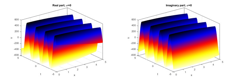
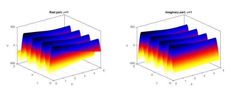
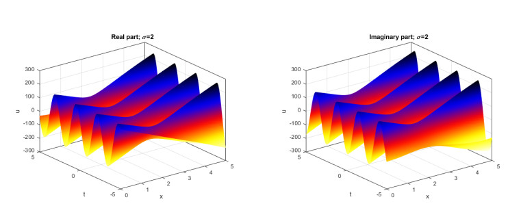
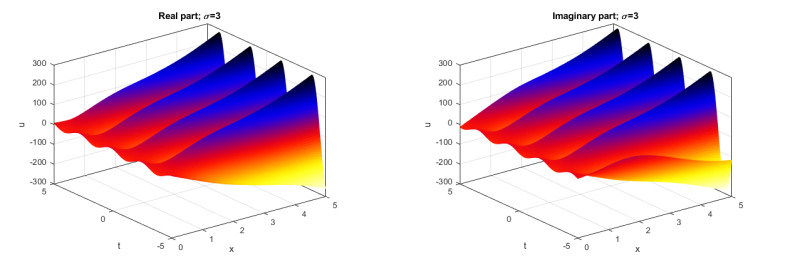
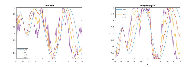
We consider in this paper the stochastic nonlinear Schrödinger equation forced by multiplicative noise in the Itô sense. We use two different methods as sine-cosine method and Riccati-Bernoulli sub-ODE method to obtain new rational, trigonometric and hyperbolic stochastic solutions. These stochastic solutions are of a qualitatively distinct nature based on the parameters. Moreover, the effect of the multiplicative noise on the solutions of nonlinear Schrödinger equation will be discussed. Finally, two and three-dimensional graphs for some solutions have been given to support our analysis.
- stochastic Schrödinger equation,
- multiplicative noise,
- exact solutions,
- sine-cosine method,
- Riccati-Bernoulli sub-ODE
Citation: Mahmoud A. E. Abdelrahman, Wael W. Mohammed, Meshari Alesemi, Sahar Albosaily. The effect of multiplicative noise on the exact solutions of nonlinear Schrödinger equation[J]. AIMS Mathematics, 2021, 6(3): 2970-2980. doi: 10.3934/math.2021180

Related Papers:

Abstract

We consider in this paper the stochastic nonlinear Schrödinger equation forced by multiplicative noise in the Itô sense. We use two different methods as sine-cosine method and Riccati-Bernoulli sub-ODE method to obtain new rational, trigonometric and hyperbolic stochastic solutions. These stochastic solutions are of a qualitatively distinct nature based on the parameters. Moreover, the effect of the multiplicative noise on the solutions of nonlinear Schrödinger equation will be discussed. Finally, two and three-dimensional graphs for some solutions have been given to support our analysis.

References

[1]	M. A. E. Abdelrahman, Global solutions for the ultra-relativistic Euler equations, Nonlinear Anal., 155 (2017), 140–162. doi: 10.1016/j.na.2017.01.014
[2]	C. O. Alves, F. Gao, M. Squassina, M. Yang, Singularly perturbed critical Choquard equations, J. Differ. Equations, 263 (2017), 3943–3988. doi: 10.1016/j.jde.2017.05.009
[3]	P. I. Naumkin, J. J. Perez, Higher-order derivative nonlinear Schrödinger equation in the critical case, J. Math. Phys., 59 (2018), 021506. doi: 10.1063/1.5008500
[4]	M. A. E. Abdelrahman, Cone-grid scheme for solving hyperbolic systems of conservation laws and one application, Comput. Appl. Math., 37 (2018), 3503–3513. doi: 10.1007/s40314-017-0527-9
[5]	M. A. E. Abdelrahman, G. M. Bahaa, Elementary waves, Riemann problem, Riemann invariants and new conservation laws for the pressure gradient model, Eur. Phys. J. Plus, 134 (2019), 187. doi: 10.1140/epjp/i2019-12580-7
[6]	M. A. E. Abdelrahman, N. F. Abdo, On the nonlinear new wave solutions in unstable dispersive environments, Phys. Scripta, 95 (2020), 045220. doi: 10.1088/1402-4896/ab62d7
[7]	H. G. Abdelwahed, Nonlinearity contributions on critical MKP equation, J. Taibah Univ. Sci., 14 (2020), 777–782. doi: 10.1080/16583655.2020.1774136
[8]	H. G. Abdelwahed, Super electron acoustic propagations in critical plasma density, J. Taibah Univ. Sci., 14 (2020), 1363–1368. doi: 10.1080/16583655.2020.1822653
[9]	M. K. Sharaf, E. K. El-Shewy, M. A. Zahran, Fractional anisotropic diffusion equation in cylindrical brush model, J. Taibah Univ. Sci., 14 (2020), 1416–1420. doi: 10.1080/16583655.2020.1824743
[10]	A. M. Wazwaz, The integrable time-dependent sine-Gordon with multiple optical kink solutions, Optik, 182 (2019), 605–610. doi: 10.1016/j.ijleo.2019.01.018
[11]	M. A. E. Abdelrahman, M. A. Sohaly, On the new wave solutions to the MCH equation, Indian J. Phys., 93 (2019), 903–911. doi: 10.1007/s12648-018-1354-6
[12]	M. Eslami, Trial solution technique to chiral nonlinear Schrödinger's equation in (1 + 2)-dimensions, Nonlinear Dyn., 85 (2016), 813–816. doi: 10.1007/s11071-016-2724-2
[13]	M. Mirzazadeh, M. Eslami, A. Biswas, 1-Soliton solution of KdV equation, Nonlinear Dyn., 80 (2015), 387–396. doi: 10.1007/s11071-014-1876-1
[14]	B. Ghanbari, C. K. Kuo, New exact wave solutions of the variable-coefficient (1 + 1)-dimensional Benjamin-Bona-Mahony and (2 + 1)-dimensional asymmetric Nizhnik-Novikov-Veselov equations via the generalized exponential rational function method, Eur. Phys. J. Plus, 134 (2019), 134. doi: 10.1140/epjp/i2019-12635-9
[15]	C. K. Kuo, B. Ghanbari, Resonant multi-soliton solutions to new (3 + 1)-dimensional Jimbo-Miwa equations by applying the linear superposition principle, Nonlinear Dyn., 96 (2019), 459–464. doi: 10.1007/s11071-019-04799-9
[16]	M. A. E. Abdelrahman, M. A. Sohaly, The development of the deterministic nonlinear PDEs in particle physics to stochastic case, Results Phys., 9 (2018), 344–350. doi: 10.1016/j.rinp.2018.02.032
[17]	M. A. E. Abdelrahman, S. Z. Hassan, M. Inc, The coupled nonlinear Schrödinger-type equations, Mod. Phys. Lett. B, 34 (2020), 2050078.
[18]	W. W. Mohammed, Amplitude equation with quintic nonlinearities for the generalized Swift-Hohenberg equation with additive degenerate noise, Adv. Differ. Equ., 1 (2016), 84.
[19]	W. W. Mohammed, Approximate solution of the Kuramoto-Shivashinsky equation on an unbounded domain, Chinese Ann. Math. B, 39 (2018), 145–162. doi: 10.1007/s11401-018-1057-5
[20]	W. W. Mohammed, Modulation equation for the stochastic Swift–Hohenberg equation with cubic and quintic nonlinearities on the real line, Mathematics, 6 (2020), 1–12.
[21]	H. G. Abdelwahed, E. K. El-Shewy, M. A. E. Abdelrahman, R. Sabry, New super waveforms for modified Korteweg-de-Veries-equation, Results Phys., 19 (2020), 103420. doi: 10.1016/j.rinp.2020.103420
[22]	N. W. Ashcroft, N. D. Mermin, Solid state physics, New York: Cengage Learning, 1976.
[23]	H. T. Chu, Eigen energies and eigen states of conduction electrons in pure bismithunder size and magnetic fields quatizations, J. Phys. Chem. Solids, 50 (1989), 319–324. doi: 10.1016/0022-3697(89)90494-0
[24]	P. I. Kelley, Self-focusing of optical beams, Phys. Rev. Lett., 15 (1965), 1005–1008. doi: 10.1103/PhysRevLett.15.1005
[25]	M. Blencowe, Quantum electromechanical systems, Phys. Rep., 395 (2004), 159–222. doi: 10.1016/j.physrep.2003.12.005
[26]	W. Grecksch, H. Lisei, Stochastic nonlinear equations of Schrödinger type, Stoch. Anal. Appl., 29 (2011), 631–653. doi: 10.1080/07362994.2011.581091
[27]	C. H. Bruneau, L. Di Menza, T. Lehner, Numerical resolution of some nonlinear Schrödinger-like equations in plasmas, Numer. Meth. Part. D. E., 15 (1999), 672–696. doi: 10.1002/(SICI)1098-2426(199911)15:6<672::AID-NUM5>3.0.CO;2-J
[28]	V. Barbu, M. Röckner, D. Zhang, Stochastic nonlinear Schrödinger equations with linear multiplicative noise: rescaling approach, J. Nonlin. Sci., 24 (2014), 383–409. doi: 10.1007/s00332-014-9193-x
[29]	M. A. E. Abdelrahman, W. W. Mohammed, The impact of multiplicative noise on the solution of the Chiral nonlinear Schrödinger equation, Phys. Scripta, 95 (2020), 085222. doi: 10.1088/1402-4896/aba3ac
[30]	S. Albosaily, W. W. Mohammed, M. A. Aiyashi, M. A. E. Abdelrahman, Exact solutions of the (2 + 1)-dimensional stochastic chiral nonlinear Schrödinger equation, Symmetry, 12 (2020), 1874. doi: 10.3390/sym12111840
[31]	A. Debussche, C. Odasso, Ergodicity for a weakly damped stochastic nonlinear Schrödinger equation, J. Evol. Equ., 5 (2005), 317–356. doi: 10.1007/s00028-005-0195-x
[32]	G. E. Falkovich, I. Kolokolov, V. Lebedev, S. K. Turitsyn, Statistics of soliton-bearing systems with additive noise, Phys. Rev. E, 63 (2001), 025601.
[33]	A. Debussche, L. Di Menzab, Numerical simulation of focusing stochastic nonlinear Schrödinger equations, Physica D, 162 (2002), 131–154. doi: 10.1016/S0167-2789(01)00379-7
[34]	K. Cheung, R. Mosincat, Stochastic nonlinear Schrö dinger equations on tori, Stoch. Partial Differ., 7 (2019), 169–208.
[35]	A. De Bouard, A. Debussche, A semidiscrete scheme for the stochastic nonlinear Schrödinger equation, Numer. Math., 96 (2004), 733–770. doi: 10.1007/s00211-003-0494-5
[36]	J. Cui, J. Hong, Z. Liu, Strong convergence rate of finite difference approximations for stochastic cubic Schrödinger equations, J. Differ. Equations, 263 (2017), 3687–3713. doi: 10.1016/j.jde.2017.05.002
[37]	J. Cui, J. Hong, Z. Liu, W. Zhou, Strong convergence rate of splitting schemes for stochastic nonlinear Schrödinger equation, J. Differ. Equations, 266 (2019), 5625–5663. doi: 10.1016/j.jde.2018.10.034
[38]	X. F. Yang, Z. C. Deng, Y. Wei, A Riccati-Bernoulli sub-ODE method for nonlinear partial differential equations and its application, Adv. Differ. Equ., 1 (2015), 117–133.
[39]	A. M. Wazwaz, A sine-cosine method for handling nonlinear wave equations, Math. Comput. Model., 40 (2004), 499–508. doi: 10.1016/j.mcm.2003.12.010
[40]	A. M. Wazwaz, The sine-cosine method for obtaining solutions with compact and noncompact structures, Appl. Math. Comput., 159 (2004), 559–576
[41]	E. Yusufoglu, A. Bekir, Solitons and periodic solutions of coupled nonlinear evolution equations by using sine-cosine method, Int. J. Comput. Math., 83 (2006), 915–924. doi: 10.1080/00207160601138756

Reader Comments

Your name:*

Email:*
© 2021 the Author(s), licensee AIMS Press. This is an open access article distributed under the terms of the Creative Commons Attribution License (http://creativecommons.org/licenses/by/4.0)