The extended Burr-R class: properties, applications and modified test for censored data

Abdulhakim A. Al-Babtain; Rehan A. K. Sherwani; Ahmed Z. Afify; Khaoula Aidi; M. Arslan Nasir; Farrukh Jamal; Abdus Saboor; Abdulhakim A. Al-Babtain; Rehan A. K. Sherwani; Ahmed Z. Afify; Khaoula Aidi; M. Arslan Nasir; Farrukh Jamal; Abdus Saboor

doi:10.3934/math.2021176

AIMS Mathematics

2021, Volume 6, Issue 3: 2912-2931. doi: 10.3934/math.2021176

Previous Article Next Article

Research article

The extended Burr-R class: properties, applications and modified test for censored data

1.
Department of Statistics and Operations Research, King Saud University, Riyadh 11362, Saudi Arabia
2.
College of Statistical and Actuarial Sciences, University of the Punjab Lahore, Pakistan
3.
Department of Statistics, Mathematics and Insurance, Benha University, Benha 13511, Egypt
4.
Laboratory of probability and statistics LaPS, University Badji Mokhtar-Annaba, Algeria
5.
Government S. E College Bahawalpur, Punjab, Pakistan
6.
Department of Statistics, The Islamia University Bahawalpur, Bahawalpur, Pakistan
7.
Kohat University of Science and Technology, KPK, Pakistan

Received: 24 October 2020 Accepted: 29 December 2020 Published: 08 January 2021
MSC : 60E05, 62F10

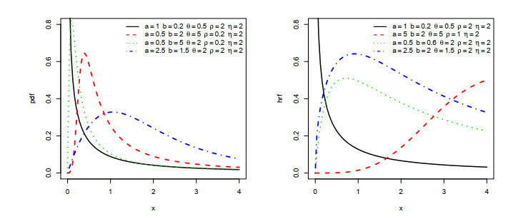
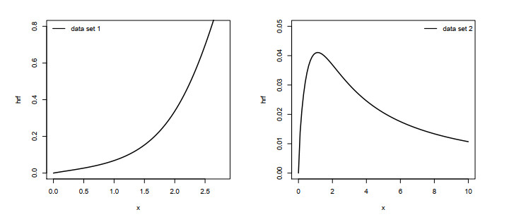
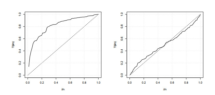
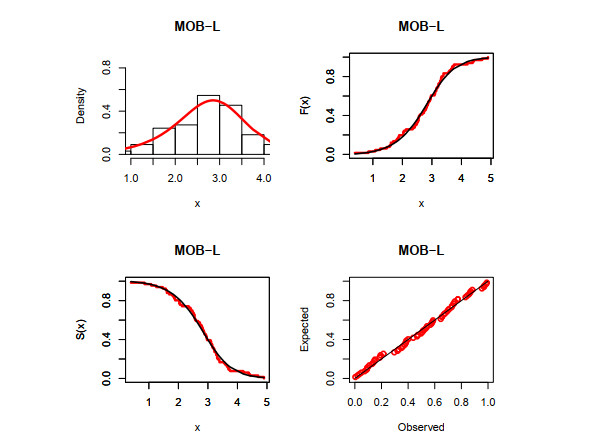
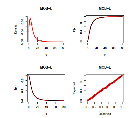
This article introduces a new three-parameter Marshall-Olkin Burr-R (MOB-R) family which extends the generalize Burr-G class. Some of its general properties are discussed. One of its special models called the MOB-Lomax distribution is studied in detail for illustrative purpose. A modified chi-square test statistic is provided for right censored data from the MOB-L distribution. The model parameters are estimated via the maximum likelihood and simulation results are obtained to assess the behavior of the maximum likelihood approach. Applications to real data sets are provided to show the usefulness of the proposed MOB-Lomax distribution. The modified chi-square test statistic shows that the MOB-Lomax model can be used as a good candidate for analyzing real censored data.
- censored data,
- Lomax distribution,
- maximum likelihood estimation,
- modified chi-squared test,
- order statistics
Citation: Abdulhakim A. Al-Babtain, Rehan A. K. Sherwani, Ahmed Z. Afify, Khaoula Aidi, M. Arslan Nasir, Farrukh Jamal, Abdus Saboor. The extended Burr-R class: properties, applications and modified test for censored data[J]. AIMS Mathematics, 2021, 6(3): 2912-2931. doi: 10.3934/math.2021176

Related Papers:

Abstract

This article introduces a new three-parameter Marshall-Olkin Burr-R (MOB-R) family which extends the generalize Burr-G class. Some of its general properties are discussed. One of its special models called the MOB-Lomax distribution is studied in detail for illustrative purpose. A modified chi-square test statistic is provided for right censored data from the MOB-L distribution. The model parameters are estimated via the maximum likelihood and simulation results are obtained to assess the behavior of the maximum likelihood approach. Applications to real data sets are provided to show the usefulness of the proposed MOB-Lomax distribution. The modified chi-square test statistic shows that the MOB-Lomax model can be used as a good candidate for analyzing real censored data.

References

[1]	A. Z. Afify, G. M. Cordeiro, N. A. Ibrahim, F. Jamal, M. Elgarhy, M. A. Nasir, The Marshall–Olkin odd Burr III-G family: theory, estimation, and engineering applications, IEEE Access, (2020).
[2]	A. Z. Afify, G. M. Cordeiro, H. M. Yousof, A. Saboor, E. M. M. Ortega, The Marshall–Olkin additive Weibull distribution with variable shapes for the hazard rate, Hacettepe J. Math. Stat., 47 (2018), 365–381.
[3]	A. Z. Afify, D. Kumar, I. Elbatal, Marshall–Olkin power generalized Weibull distribution with applications in engineering and medicine, J. Stat. Theory Appl., 19 (2020), 223–237. doi: 10.2991/jsta.d.200507.004
[4]	A. Z. Afify, O. A. Mohamed, A new three–parameter exponential distribution with variable shapes for the hazard rate: estimation and applications, Mathematics, 8 (2020), 1–17. doi: 10.3390/math8101793
[5]	A. Z. Afify, M. Nassar, G. M. Cordeiro, D. Kumar, The Weibull Marshall–Olkin Lindley distribution: properties and estimation, J. Taibah Univ. Sci., 14 (2020), 192–204. doi: 10.1080/16583655.2020.1715017
[6]	A. Z. Afify, M. Zayed, M. Ahsanullah, The extended exponential distribution and its applications, J. Stat. Theory Appl., 17 (2018), 213–229. doi: 10.2991/jsta.2018.17.2.3
[7]	T. Alice, K. K. Jose, Marshall–Olkin Pareto distributions and its reliability applications, IAPQR Trans., 29 (2004), 1–9.
[8]	V. B. Bagdonavicius, R. J. Levuliene, M. S. Nikulin, Chi–square goodness-of-fit tests for parametric accelerated failure time models, Commun. Stat. Theory Methods, 42 (2013), 2768–2785. doi: 10.1080/03610926.2011.617483
[9]	V. Bagdonavicius, M. Nikulin, Chi–square goodness-of-fit test for right censored data, Int. J. Appl. Math. Stat., 24 (2011), 30–50.
[10]	G. M. Cordeiro, A. J. Lemonte, On the Marshall–Olkin extended weibull distribution, Stat. pap., 54 (2013), 333–353. doi: 10.1007/s00362-012-0431-8
[11]	G. Cordeiro, M. Mead, A. Z. Afify, A. Suzuki, A. Abd El-Gaied, An extended Burr XII distribution: properties, inference and applications, Pak. J. Stat. Oper. Res., 13 (2017), 809–828.
[12]	I. Gijbels, U. Gurler, Estimation of a change-point in a hazard function based on censored data, Lifetime Data Anal., 9 (2003), 395–411. doi: 10.1023/B:LIDA.0000012424.71723.9d
[13]	I. S. Gradshteyn, I. M. Ryzhik, Table of Integrals: Series, and Products, sixth ed., Academic Press, San Diego, 2000.
[14]	K. K. Jose, A. Joseph, M. M. Ristić, A Marshall-Olkin beta distribution and its applications, J. Prob. Stat. Sci., 7 (2009), 173–186.
[15]	E. T. Lee, J. W. Wang, Statistical Methods for Survival Data Analysis, 3rd ed., Wiley, New York, 2003.
[16]	A. W. Marshall, I. Olkin, A new method for adding a parameter to a family of distributions with application to the exponential and Weibull families, Biometrika, 84 (1997), 641–652. doi: 10.1093/biomet/84.3.641
[17]	A. J. Lemonte, G. M. Cordeiro, An extended Lomax distribution, Stat. J. Theor. Appl. Stat., 47 (2013), 800–816.
[18]	D. E. Matthews, V. T. Farewell, R. Pyke, Asymptotic score-statistic processes and tests for constant hazard against a change-point alternative, Ann. Statist., 13 (1985), 583–591.
[19]	M. E. Mead, G. M. Cordeiro, A. Z. Afify, H. Al Mofleh, The alpha power transformation family: properties and applications, Pak. J. Stat. Oper. Res., 15 (2019), 525–545.
[20]	M. A. Nasir, M. H. Tahir, F. Jamal, G. Ozel, A new generalized Burr family of distributions for the lifetime data, J. Stat. Appl. Prob., 6 (2017), 1–17. doi: 10.18576/jsap/060101
[21]	G. S. Mudholkar, D. K. Srivastava, Exponentiated Weibull family for analyzing bathtub failure-rate data, IEEE Trans. Reliab., 42 (1993), 299–302. doi: 10.1109/24.229504
[22]	M. Nassar, D. Kumar, S. Dey, G. M. Cordeiro, A. Z. Afify, The Marshall–Olkin alpha power family of distributions with applications, J. Comput. Appl. Math., 351 (2019), 41–53. doi: 10.1016/j.cam.2018.10.052
[23]	M. Shaked, J. G. Shanthikumar, Stochastic Orders, Springer: New York, NY, USA, 2007.
[24]	V. Voinov, M. Nikulin, N. Balakrishnan, Chi-square goodness of fit tests with applications, Academic Press, Elsevier, 2013.

Reader Comments

Your name:*

Email:*
© 2021 the Author(s), licensee AIMS Press. This is an open access article distributed under the terms of the Creative Commons Attribution License (http://creativecommons.org/licenses/by/4.0)