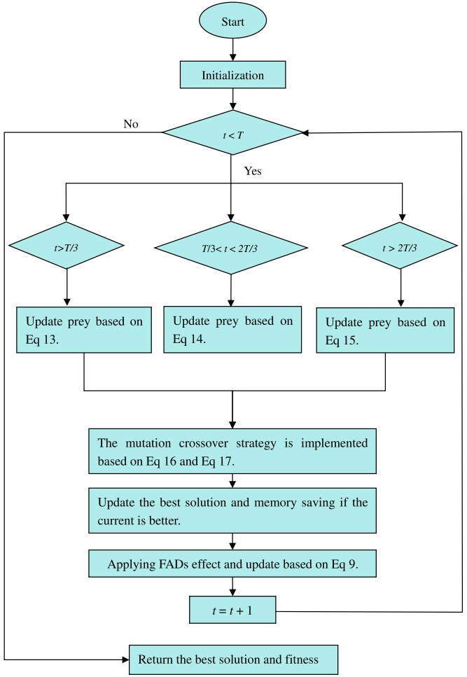
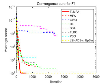
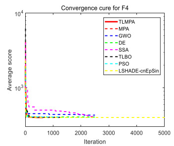
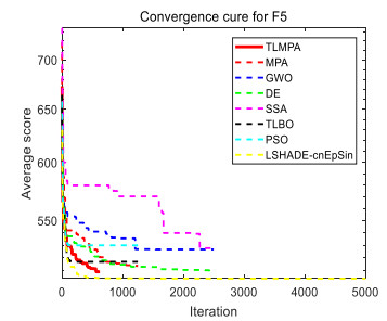
Marine Predators algorithm (MPA) is a newly proposed nature-inspired metaheuristic algorithm. The main inspiration of this algorithm is based on the extensive foraging strategies of marine organisms, namely Lévy movement and Brownian movement, both of which are based on random strategies. In this paper, we combine the marine predator algorithm with Teaching-learning-based optimization algorithm, and propose a hybrid algorithm called Teaching-learning-based Marine Predator algorithm (TLMPA). Teaching-learning-based optimization (TLBO) algorithm consists of two phases: the teacher phase and the learner phase. Combining these two phases with the original MPA enables the predators to obtain prey information for foraging by learning from teachers and interactive learning, thus greatly increasing the encounter rate between predators and prey. In addition, effective mutation and crossover strategies were added to increase the diversity of predators and effectively avoid premature convergence. For performance evaluation TLMPA algorithm, it has been applied to IEEE CEC-2017 benchmark functions and four engineering design problems. The experimental results show that among the proposed TLMPA algorithm has the best comprehensive performance and has more outstanding performance than other the state-of-the-art metaheuristic algorithms in terms of the performance measures.
Citation: Keyu Zhong, Qifang Luo, Yongquan Zhou, Ming Jiang. TLMPA: Teaching-learning-based Marine Predators algorithm[J]. AIMS Mathematics, 2021, 6(2): 1395-1442. doi: 10.3934/math.2021087
Marine Predators algorithm (MPA) is a newly proposed nature-inspired metaheuristic algorithm. The main inspiration of this algorithm is based on the extensive foraging strategies of marine organisms, namely Lévy movement and Brownian movement, both of which are based on random strategies. In this paper, we combine the marine predator algorithm with Teaching-learning-based optimization algorithm, and propose a hybrid algorithm called Teaching-learning-based Marine Predator algorithm (TLMPA). Teaching-learning-based optimization (TLBO) algorithm consists of two phases: the teacher phase and the learner phase. Combining these two phases with the original MPA enables the predators to obtain prey information for foraging by learning from teachers and interactive learning, thus greatly increasing the encounter rate between predators and prey. In addition, effective mutation and crossover strategies were added to increase the diversity of predators and effectively avoid premature convergence. For performance evaluation TLMPA algorithm, it has been applied to IEEE CEC-2017 benchmark functions and four engineering design problems. The experimental results show that among the proposed TLMPA algorithm has the best comprehensive performance and has more outstanding performance than other the state-of-the-art metaheuristic algorithms in terms of the performance measures.

| [1] | J. H. Holland, Genetic algorithms, Sci. Am., 267 (1992), 66-72. |
| [2] | J. Kennedy, R. Eberhart, Particle swarm optimization, Perth, WA, Australia: Proceedings of IEEE International Conference on Neural Networks, 1995. |
| [3] |
R. Storn, K. Price, Differential evolution-a simple and efficient heuristic for global optimization over continuous spaces, J. Global Optim., 11 (1997), 341-359. doi: 10.1023/A:1008202821328

|
| [4] | K. V. Price, Differential evolution: A fast and simple numerical optimizer, Berkeley, CA, USA: Proceedings of North American Fuzzy Information Processing, 1996. |
| [5] |
D. Karaboga, B. Basturk, A powerful and efficient algorithm for numerical function optimization: Artificial bee colony (ABC) algorithm, J. Global Optim., 39 (2007), 459-471. doi: 10.1007/s10898-007-9149-x
|
| [6] | C. R. Hwang, Simulated annealing: Theory and applications, Acta Appl. Math., 12 (1988), 108- 111. |
| [7] |
A. Faramarzi, M. Heidarinejad, S. Mirjalili, A. H. Gandomi, Marine Predators algorithm: A natureinspired metaheuristic, Expert Syst. Appl., 152 (2020), 113377. doi: 10.1016/j.eswa.2020.113377
|
| [8] | S. Mirjalili, S. M. Mirjalili, A. Lewis, Grey wolf optimizer, Adv. Eng. Software, 69 (2014), 46-61. |
| [9] | S. Mirjalili, A. Lewis, The whale optimization algorithm, Adv. Eng. Software, 95 (2016), 51-67. |
| [10] |
S. Mirjalili, A. H. Gandomi, S. Z. Mirjalili, S. Saremi, H. Faris, S. M. Mirjalili, Salp swarm algorithm: A bio-inspired optimizer for engineering design problems, Adv. Eng. Software, 114 (2017), 163-191. doi: 10.1016/j.advengsoft.2017.07.002
|
| [11] |
R. V. Rao, V. J. Savsani, D. P. Vakharia, Teaching-learning-based optimization: A novel method for constrained mechanical design optimization problems, Comput.-Aided Des., 43 (2011), 303-315. doi: 10.1016/j.cad.2010.12.015
|
| [12] |
D. H. Wolpert, W. G. Macready, No free lunch theorems for optimization, IEEE Trans. Evol. Comput., 1 (1997), 67-82. doi: 10.1109/4235.585893
|
| [13] |
M. Liu, X. Yao, Y. Li, Hybrid whale optimization algorithm enhanced with Lévy flight and differential evolution for job shop scheduling problems, Appl. Soft Comput., 87 (2020), 105954. doi: 10.1016/j.asoc.2019.105954
|
| [14] | D. Tansui, A. Thammano, Hybrid nature-inspired optimization algorithm: Hydrozoan and sea turtle foraging algorithms for solving continuous optimization problems, IEEE Access, 8 (2020), 65780- 65800. |
| [15] |
H. Garg, A hybrid GSA-GA algorithm for constrained optimization problems, Inf. Sci., 478 (2019), 499-523. doi: 10.1016/j.ins.2018.11.041
|
| [16] | D. T. Le, D. K. Bui, T. D. Ngo, Q. H. Nguyen, H. Nguyen-Xuan, A novel hybrid method combining electromagnetism-like mechanism and firefly algorithms for constrained design optimization of discrete truss structures, Comput. Struct., 212 (2019), 20-42. |
| [17] | N. E. Humphries, N. Queiroz, J. R. M. Dyer, N. G. Pade, M. K. Musyl, K. M. Schaefer, et al., Environmental context explains Lévy and Brownian movement patterns of marine predators, Nature, 465 (2010), 1066-1069. |
| [18] |
F. Bartumeus, J. Catalan, U. L. Fulco, M. L. Lyra, G. M. Viswanathan, Erratum: Optimizing the encounter rate in biological interactions: Lévy versus brownian strategies, Phys. Rev. Lett., 89 (2002), 109902. doi: 10.1103/PhysRevLett.89.109902
|
| [19] | M. A. A. Al-qaness, A. A. Ewees, H. Fan, L. Abualigah, M. A. Elaziz, Marine Predators algorithm for forecasting confirmed cases of COVID-19 in Italy, USA, Iran and Korea, Int. J. Environ. Res. Public Health, 17 (2020), 3520. |
| [20] | D. Yousri, T. S. Babu, E. Beshr, M. B. Eteiba, D. Allam, A robust strategy based on marine predators algorithm for large scale photovoltaic array reconfiguration to mitigate the partial shading effect on the performance of PV system, IEEE Access, 8 (2020), 112407-112426. |
| [21] | M. Abdel-Basset, R. Mohamed, M. Elhoseny, R. K. Chakrabortty, M. Ryan, A hybrid COVID- 19 detection model using an improved Marine Predators algorithm and a ranking-based diversity reduction strategy, IEEE Access, 8 (2020), 79521-79540. |
| [22] | M. A. Elaziz, A. A. Ewees, D. Yousri, H. S. N. Alwerfali, Q. A. Awad, S. Lu, et al., An improved Marine Predators algorithm with fuzzy entropy for multi-level thresholding: Real world example of COVID-19 CT image segmentation, IEEE Access, 8 (2020), 125306-125330. |
| [23] |
R. V. Rao, V. Patel, Multi-objective optimization of heat exchangers using a modified teachinglearning-based optimization algorithm, Appl. Math. Modell., 37 (2013), 1147-1162. doi: 10.1016/j.apm.2012.03.043
|
| [24] | R. V. Rao, V. Patel, An improved Teaching-learning-based optimization algorithm for solving unconstrained optimization problems, Sci. Iran., 20 (2013), 710-720. |
| [25] |
A. R. Yildiz, Optimization of multi-pass turning operations using hybrid teaching learning-based approach, Int. J. Adv. Manuf. Technol., 66 (2013), 1319-1326. doi: 10.1007/s00170-012-4410-y
|
| [26] |
K. Yu, X. Wang, Z. Wang, An improved Teaching-learning-based optimization algorithm for numerical and engineering optimization problems, J. Intell. Manuf., 27 (2016), 831-843. doi: 10.1007/s10845-014-0918-3
|
| [27] | E. Uzlu, M. Kankal, A. Akpınar, T. Dede, Estimates of energy consumption in Turkey using neural networks with the Teaching-learning-based optimization algorithm, Energy, 75 (2014), 295-303. |
| [28] | V. Toǧan, Design of planar steel frames using teaching-learning based optimization, Eng. Struct., 34 (2012), 225-232. |
| [29] |
R. V. Rao, V. D. Kalyankar, Parameter optimization of modern machining processes using teachinglearning-based optimization algorithm, Eng. Appl. Artif. Intell., 26 (2013), 524-531. doi: 10.1016/j.engappai.2012.06.007
|
| [30] |
M. Singh, B. K. Panigrahi, A. R. Abhyankar, S. Das, Optimal coordination of directional overcurrent relays using informative differential evolution algorithm, J. Comput. Sci., 5 (2014), 269-276. doi: 10.1016/j.jocs.2013.05.010
|
| [31] |
H. Bouchekara, M. A. Abido, M. Boucherma, Optimal power flow using Teaching-learning-based optimization technique, Electr. Power Syst. Res., 114 (2014), 49-59. doi: 10.1016/j.epsr.2014.03.032
|
| [32] | G. M. Viswanathan, V. Afanasyev, S. V. Buldyrev, E. J. Murphy, P. A. Prince, H. E. Stanley, Lévy flight search patterns of wandering albatrosses, Nature, 381 (1996), 413-415. |
| [33] | J. D. Filmalter, L. Dagorn, P. D. Cowley, M. Taquet, First descriptions of the behavior of silky sharks, Carcharhinus falciformis, around drifting fish aggregating devices in the Indian Ocean, Bull. Mar. Sci., 87 (2011), 325-337. |
| [34] | E. Clark, Instrumental conditioning of lemon sharks, Science (New York, N.Y.), 130 (1959), 217-218. |
| [35] | L. A. Dugatkin, D. S. Wilson, The prerequisites for strategic behaviour in bluegill sunfish, Lepomis macrochirus, Anim. Behav., 44 (1992), 223-230. |
| [36] | V. Schluessel, H. Bleckmann, Spatial learning and memory retention in the grey bamboo shark (Chiloscyllium griseum), Zoology, 115 (2012), 346-353. |
| [37] | D. W. Zimmerman, B. D. Zumbo, Relative power of the Wil-coxon test, the Friedman test, and repeated-measures ANOVA on ranks, J. Exp. Educ., 62 (1993), 75-86. |
| [38] | S. Mirjalili, A. H. Gandomi, S. Z. Mirjalili, S. Saremi, H. Faris, S. M. Mirjalili, Salp swarm algorithm: A bio-inspired optimizer for engineering design problems, Adv. Eng. Software, 114 (2017), 163-191. |
| [39] |
C. A. C. Coello, E. M. Montes, Constraint-handling in genetic algorithms through the use of dominance-based tournament selection, Adv. Eng. Inf., 16 (2002), 193-203. doi: 10.1016/S1474-0346(02)00011-3
|
| [40] |
E. Rashedi, H. Nezamabadi-pour, S. Saryazdi, GSA: A gravitational search algorithm, Inf. Sci., 179 (2009), 2232-2248. doi: 10.1016/j.ins.2009.03.004
|
| [41] | H. Eskandar, A. Sadollah, A. Bahreininejad, M. Hamdi, Water cycle algorithm-a novel metaheuristic optimization method for solving constrained engineering optimization problems, Comput. Struct., 110 (2012), 151-166. |
| [42] | R. A. Krohling, L. dos Santos Coelho, Coevolutionary particle swarm optimization using Gaussian distribution for solving constrained optimization problems, IEEE Trans. Syst., Man, Cybern., Part B (Cybernetics), 36 (2006), 1407-1416. |
| [43] |
K. M. Ragsdell, D. T. Phillips, Optimal design of a class of welded structures using geometric programming, J. Eng. Ind., 98 (1976), 1021-1025. doi: 10.1115/1.3438995
|
| [44] |
P. Savsani, V. Savsani, Passing vehicle search (PVS): A novel metaheuristic algorithm, Appl. Math. Model., 40 (2016), 3951-3978. doi: 10.1016/j.apm.2015.10.040
|
| [45] | M. Dorigo, T. Stützle, Ant colony optimization: Overview and recent advances, 2Eds., Cham, Switzerland: Springer International Publishing, 2019. |
| [46] | S. Mirjalili, A. Lewis, The whale optimization algorithm, Adv. Eng. Software, 95 (2016), 51-67. |
| [47] |
S. Mirjalili, SCA: A sine cosine algorithm for solving optimization problems, Knowl.-Based Syst., 96 (2016), 120-133. doi: 10.1016/j.knosys.2015.12.022
|
| [48] |
H. Beyer, H. Schwefel, Evolution strategies-A comprehensive introduction, Nat. Comput., 1 (2002), 3-52. doi: 10.1023/A:1015059928466
|
| [49] |
R. Moghdani, K. Salimifard, Volleyball premier league algorithm, Appl. Soft Comput., 64 (2018), 161-185. doi: 10.1016/j.asoc.2017.11.043
|
| [50] |
H. Liu, Z. Cai, Y. Wang, Hybridizing particle swarm optimization with differential evolution for constrained numerical and engineering optimization, Appl. Soft Comput., 10 (2010), 629-640. doi: 10.1016/j.asoc.2009.08.031
|
| [51] |
K. Thirugnanasambandam, S. Prakash, V. Subramanian, S. Pothula, V. Thirumal, Reinforced cuckoo search algorithm-based multimodal optimization, Appl. Intell., 49 (2019), 2059-2083. doi: 10.1007/s10489-018-1355-3
|
| [52] | K. Deb, GeneAS: A robust optimal design technique for mechanical component design, 2Eds., Berlin, Heidelberg: Springer Berlin Heidelberg, 1997. |
| [53] | M. Mahdavi, M. Fesanghary, E. Damangir, An improved harmony search algorithm for solving optimization problems, Appl. Math. Comput., 188 (2007), 1567-1579. |
| [54] | E. Mezura-Montes, C. A. C. Coello, R. Landa-Becerra, Engineering optimization using simple evolutionary algorithm, Sacramento, CA, USA: Proceedings. 15th IEEE International Conference on Tools with Artificial Intelligence, 2003. |
| [55] |
T. Ray, P. Saini, Engineering design optimization using swarm with an intelligent information sharing among individuals, Eng. Optim., 33 (2001), 735-748. doi: 10.1080/03052150108940941
|
| [56] |
A. D. Belegundu, J. S. Arora, A study of mathematical programming methods for structural optimization. Part I: Theory, Int. J. Numer. Methods Eng., 21 (1985), 1583-1599. doi: 10.1002/nme.1620210904
|
| [57] |
T. Ray, K. M. Liew, Society and civilization: An optimization algorithm based on the simulation of social behavior, IEEE Trans. Evol. Comput., 7 (2003), 386-396. doi: 10.1109/TEVC.2003.814902
|
| [58] | Q. Zhang, H. Chen, A. A. Heidari, X. Zhao, Y. Xu, P. Wang, et al., Chaos-induced and mutationdriven schemes boosting salp chains-inspired optimizers, IEEE Access, 7 (2019), 31243-31261. |
| [59] | A. Kaveh, M. Khayatazad, A new meta-heuristic method: Ray optimization, Comput. Struct., 112 (2012), 283-294. |
| [60] | F. Huang, L. Wang, Q. He, An effective co-evolutionary differential evolution for constrained optimization, Appl. Math. Comput., 186 (2007), 340-356. |
| [61] |
E. M. Montes, C. A. C. Coello, An empirical study about the usefulness of evolution strategies to solve constrained optimization problems, Int. J. Gen. Syst., 37 (2008), 443-473. doi: 10.1080/03081070701303470
|
| [62] |
S. Mirjalili, Moth-flame optimization algorithm: a novel nature-inspired heuristic paradigm, Knowl.-Based Syst., 89 (2015), 228-249. doi: 10.1016/j.knosys.2015.07.006
|
| [63] | J. S. Arora, Introduction to optimum design, New York: McGraw-Hill Book Co., 1989. |
| [64] |
A. A. Heidari, R. A. Abbaspour, A. R. Jordehi, An efficient chaotic water cycle algorithm for optimization tasks, Neural Comput. Appl., 28 (2017), 57-85. doi: 10.1007/s00521-015-2037-2
|
| [65] |
A. H. Gandomi, X. S. Yang, A. H. Alavi, S. Talatahari, Bat algorithm for constrained optimization tasks, Neural Comput. Appl., 22 (2013), 1239-1255. doi: 10.1007/s00521-012-1028-9
|
| [66] |
H. Rosenbrock, An automatic method for finding the greatest or least value of a function, Comput. J., 3 (1960), 175-184. doi: 10.1093/comjnl/3.3.175
|
| [67] | L. dos Santos Coelho, Gaussian quantum-behaved particle swarm optimization approaches for constrained engineering design problems, Expert Syst. Appl., 37 (2010), 1676-1683. |
| [68] |
E. Mezura-Montes, C. A. C. Coello, A simple multimembered evolution strategy to solve constrained optimization problems, IEEE Trans. Evol. Comput., 9 (2005), 1-17. doi: 10.1109/TEVC.2004.836819
|
| [69] | F. Huang, L. Wang, Q. He, An effective co-evolutionary differential evolution for constrained optimization, Appl. Math. Comput., 186 (2007), 340-356. |
| [70] |
M. Montemurro, A. Vincenti, P. Vannucci, The automatic dynamic penalisation method (ADP) for handling constraints with genetic algorithms, Comput. Methods Appl. Mech. Eng., 256 (2013), 70-87. doi: 10.1016/j.cma.2012.12.009
|
| [71] |
K. Deb, Optimal design of a welded beam via genetic algorithms, AIAA J., 29 (1991), 2013-2015. doi: 10.2514/3.10834
|
| [72] |
A. Kaveh, S. Talatahari, A novel heuristic optimization method: Charged system search, Acta Mech., 213 (2010), 267-289. doi: 10.1007/s00707-009-0270-4
|
| [73] |
B. K. Kannan, S. N. Kramer, An augmented lagrange multiplier based method for mixed integer discrete continuous optimization and its applications to mechanical design, J. Mech. Des., 116 (1994), 405-411. doi: 10.1115/1.2919393
|
| [74] |
C. Ozturk, E. Hancer, D. Karaboga, Dynamic clustering with improved binary artificial bee colony algorithm, Appl. Soft Comput., 28 (2015), 69-80. doi: 10.1016/j.asoc.2014.11.040
|
| [75] |
X. Kong, L. Gao, H. Ouyang, S. Li, A simplified binary harmony search algorithm for large scale 0-1 knapsack problems, Expert Syst. Appl., 42 (2015), 5337-5355. doi: 10.1016/j.eswa.2015.02.015
|
| [76] |
M. Abdel-Basset, D. El-Shahat, H. Faris, S. Mirjalili, A binary multi-verse optimizer for 0-1 multidimensional knapsack problems with application in interactive multimedia systems, Comput. Ind. Eng., 132 (2019), 187-206. doi: 10.1016/j.cie.2019.04.025
|
| [77] |
P. Brucker, R. Qu, E. K. Burke, Personnel scheduling: Models and complexity, Eur. J. Oper. Res., 210 (2011), 467-473. doi: 10.1016/j.ejor.2010.11.017
|
| [78] |
M. M. Solomon, Algorithms for the vehicle routing and scheduling problems with time window constraints, Oper. Res., 35 (1987), 254-265. doi: 10.1287/opre.35.2.254
|
| [79] |
P. V. Laarhoven, E. Aarts, J. K. Lenstra, Job shop scheduling by simulated annealing, Oper. Res., 40 (1992), 113-125. doi: 10.1287/opre.40.1.113
|
| [80] | J. Zhang, J. Zhang, T. Lok, M. R. Lyu, A hybrid particle swarm optimization-back-propagation algorithm for feedforward neural network training, Appl. Math. Comput., 185 (2007), 1026-1037. |
| [81] |
K. Socha, C. Blum, An ant colony optimization algorithm for continuous optimization: Application to feed-forward neural network training, Neural Comput. Appl., 16 (2007), 235-247. doi: 10.1007/s00521-007-0084-z
|
| [82] | K. Y. Leong, A. Sitiol, K. S. M. Anbananthen, Enhance neural networks training using GA with chaos theory, 3Eds., Berlin, Heidelberg: Springer Berlin Heidelberg, 2009. |
| [83] |
X. Wang, J. Yang, X. Teng, W. Xia, R. Jensen, Feature selection based on rough sets and particle swarm optimization, Pattern Recognit. Lett., 28 (2007), 459-471. doi: 10.1016/j.patrec.2006.09.003
|
| [84] | M. Ghaemi, M. R. Feizi-Derakhshi, Feature selection using forest optimization algorithm, Pattern Recognit., 60 (2016), 121-129. |
| [85] |
P. R. Varma, V. V. Kumari, S. S. Kumar, Feature selection using relative fuzzy entropy and ant colony optimization applied to real-time intrusion detection system, Procedia Comput. Sci., 85 (2016), 503-510. doi: 10.1016/j.procs.2016.05.203
|


Figures(33) / Tables(20)

Keyu Zhong, Qifang Luo, Yongquan Zhou, Ming Jiang. TLMPA: Teaching-learning-based Marine Predators algorithm[J]. AIMS Mathematics, 2021, 6(2): 1395-1442. doi: 10.3934/math.2021087


 DownLoad: