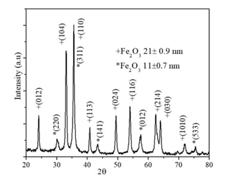
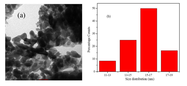
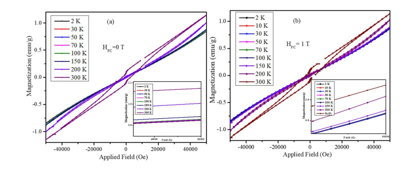
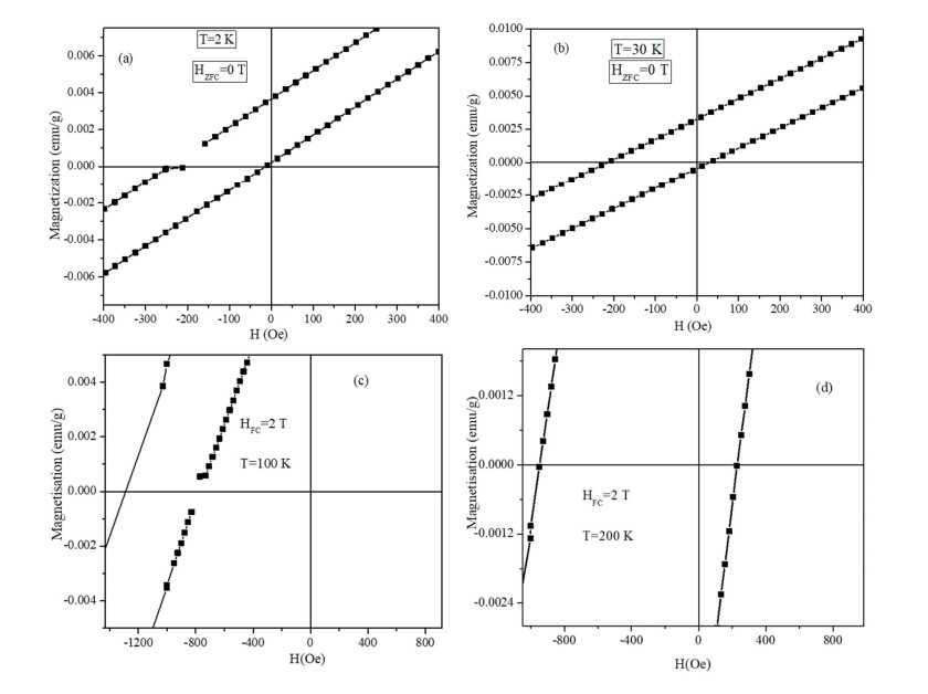
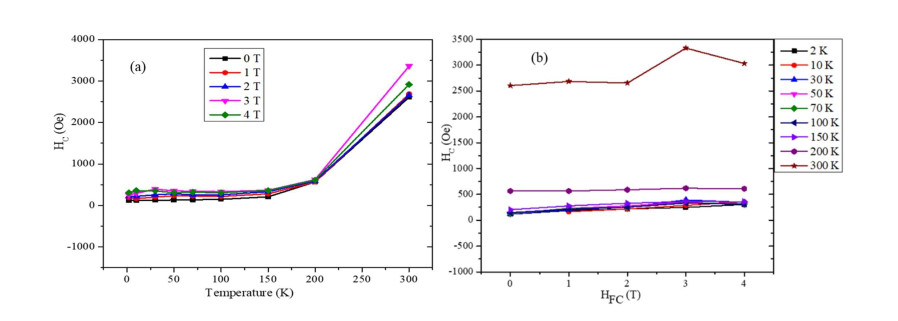
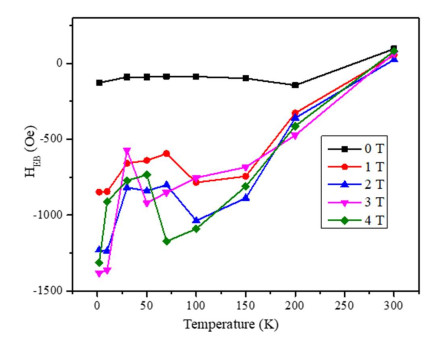
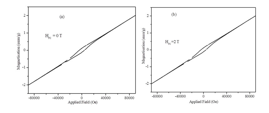
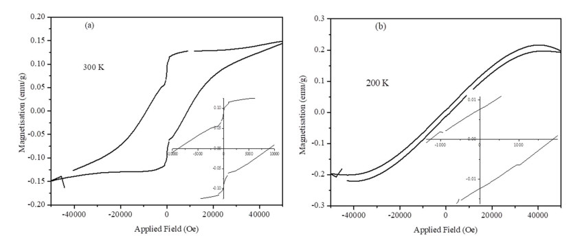
Hematite nanoparticles of average size of 20 nm were synthesized using sol-gel method and the structural characterisations were conducted using XRD and TEM. The XRD profile revealed the coexistence of small fraction of maghemite phase along with the main hematite phase. Magnetization versus applied field (M-H) measurements were performed between −5 and 5 T and respectively in the temperatures 2, 10, 30, 50, 70,100,150,200, and 300 K under zero field and 1, 2, 3, 4 T field cooling. At all field-cooling values, the coercivity was found to display a weak temperatures dependence below 150 K and a strong increase above 150 K reaching the largest value of 3352 Oe at 300 K for the field-cooling value of 3 T. Horizontal and vertical hysteresis loop shifts were observed at all temperatures in both the zero-field and field-cooled states. In the field-cooled state, both loop shifts where found to have significant and nonmonotonic field-cooling dependences. However, because saturation magnetization was not attained in all measurements our calculations were based on the minor hysteresis loops. M-H measurements were performed between −9 and 9 T at room temperature under zero field cooling and 1, 2, 3, 4, 5, 6 T field cooling. Saturation magnetization was not attained, and the loops displayed loop shifts similar to those for the ±5 T sweeping field. The highest coercivity value of 4400 Oe is observed for the 6 T field cooled MH loop. The ferromagnetic (FM) contribution towards the total magnetization was separated from the total magnetization and hysteresis loops displayed both horizontal and vertical shifts. The novel results of the temperature and field dependence of exchange bias were attributed mainly to the magnetic exchange coupling between the different magnetic phases (mainly the FM) and the spin-glass-like regions.
Citation: Venkatesha Narayanaswamy, Imaddin A. Al-Omari, Aleksandr. S. Kamzin, Chandu V. V. Muralee Gopi, Abbas Khaleel, Sulaiman Alaabed, Bashar Issa, Ihab M. Obaidat. Exchange bias, and coercivity investigations in hematite nanoparticles[J]. AIMS Materials Science, 2022, 9(1): 71-84. doi: 10.3934/matersci.2022005
Hematite nanoparticles of average size of 20 nm were synthesized using sol-gel method and the structural characterisations were conducted using XRD and TEM. The XRD profile revealed the coexistence of small fraction of maghemite phase along with the main hematite phase. Magnetization versus applied field (M-H) measurements were performed between −5 and 5 T and respectively in the temperatures 2, 10, 30, 50, 70,100,150,200, and 300 K under zero field and 1, 2, 3, 4 T field cooling. At all field-cooling values, the coercivity was found to display a weak temperatures dependence below 150 K and a strong increase above 150 K reaching the largest value of 3352 Oe at 300 K for the field-cooling value of 3 T. Horizontal and vertical hysteresis loop shifts were observed at all temperatures in both the zero-field and field-cooled states. In the field-cooled state, both loop shifts where found to have significant and nonmonotonic field-cooling dependences. However, because saturation magnetization was not attained in all measurements our calculations were based on the minor hysteresis loops. M-H measurements were performed between −9 and 9 T at room temperature under zero field cooling and 1, 2, 3, 4, 5, 6 T field cooling. Saturation magnetization was not attained, and the loops displayed loop shifts similar to those for the ±5 T sweeping field. The highest coercivity value of 4400 Oe is observed for the 6 T field cooled MH loop. The ferromagnetic (FM) contribution towards the total magnetization was separated from the total magnetization and hysteresis loops displayed both horizontal and vertical shifts. The novel results of the temperature and field dependence of exchange bias were attributed mainly to the magnetic exchange coupling between the different magnetic phases (mainly the FM) and the spin-glass-like regions.

| [1] |
Colombo M, Carregal S, Casula MF, et al. (2012) Biological applications of magnetic nanoparticles. Chem Soc Rev 41: 4306-4334. https://doi.org/10.1039/c2cs15337h doi: 10.1039/c2cs15337h

|
| [2] |
Angelakeris M (2017) Magnetic nanoparticles: A multifunctional vehicle for modern theranostics. BBA Gen Subjects 1861: 1642-1651. https://doi.org/10.1016/j.bbagen.2017.02.022 doi: 10.1016/j.bbagen.2017.02.022
|
| [3] |
Issa B, Qadri S, Obaidat IM, et al. (2011) PEG coating reduces NMR relaxivity of Mn0.5Zn0.5Gd0.02Fe1.98O4 hyperthermia nanoparticles. J Magn Reson Imaging 34: 1192-1198. https://doi.org/10.1002/jmri.22703 doi: 10.1002/jmri.22703
|
| [4] |
Atabaev TS, Vu HHT, Ajmal M, et al. (2015) Dual-mode spectral convertors as a simple approach for the enhancement of hematite's solar water splitting efficiency. Appl Phys A-Mater 119: 1373-1377. https://doi.org/10.1007/s00339-015-9108-1 doi: 10.1007/s00339-015-9108-1
|
| [5] |
Boutchuen A, Zimmerman D, Aich N, et al. (2019) Increased plant growth with hematite nanoparticle fertilizer drop and determining nanoparticle uptake in plants using multimodal approach. J Nanomater 2019: e6890572. https://doi.org/10.1155/2019/6890572 doi: 10.1155/2019/6890572
|
| [6] |
Obaidat IM, Mohite V, Issa B, et al. (2009) Predicting a major role of surface spins in the magnetic properties of ferrite nanoparticles. Cryst Res Technol 44: 489-494. https://doi.org/10.1002/crat.200900022 doi: 10.1002/crat.200900022
|
| [7] |
Obaidat IM, Issa B, Haik Y (2011) The role of aggregation of ferrite nanoparticles on their magnetic properties. J Nanosci Nanotechnol 11: 3882-3888. https://doi.org/10.1166/jnn.2011.3833 doi: 10.1166/jnn.2011.3833
|
| [8] |
Bañobre LM, Teijeiro A, Rivas J (2013) Magnetic nanoparticle-based hyperthermia for cancer treatment. Rep Pract Oncol Radiother 18: 397-400. https://doi.org/10.1016/j.rpor.2013.09.011 doi: 10.1016/j.rpor.2013.09.011
|
| [9] | Laurent S, Elst LV, Muller RN (2013) Superparamagnetic iron oxide nanoparticles for MRI, In: The Chemistry of Contrast Agents in Medical Magnetic Resonance Imaging, 2 Eds., New York: John Wiley & Sons, 427-447. https://doi.org/10.1002/9781118503652.ch10 |
| [10] | Cornell RM, Schwertmann U (2003) The Iron Oxides: Structure, Properties, Reactions, Occurrences and Uses, 2 Eds., New York: John Wiley & Sons. https://doi.org/10.1002/3527602097 |
| [11] |
Demortière A, Panissod P, Pichon BP, et al. (2011) Size-dependent properties of magnetic iron oxide nanocrystals. Nanoscale 3: 225-232. https://doi.org/10.1039/C0NR00521E doi: 10.1039/C0NR00521E
|
| [12] |
Ashraf M, Khan I, Usman M, et al. (2020) Hematite and magnetite nanostructures for green and sustainable energy harnessing and environmental pollution control: a review. Chem Res Toxicol 33: 1292-1311. https://doi.org/10.1021/acs.chemrestox.9b00308 doi: 10.1021/acs.chemrestox.9b00308
|
| [13] |
Xue Y, Wang Y (2020) A review of the α-Fe2O3 (hematite) nanotube structure: recent advances in synthesis, characterization, and applications. Nanoscale 12: 10912-10932. https://doi.org/10.1039/D0NR02705G doi: 10.1039/D0NR02705G
|
| [14] |
Liu J, Yang H, Xue X (2019) Preparation of different shaped α-Fe2O3 nanoparticles with large particles of iron oxide red. CrystEngComm 21: 1097-1101. https://doi.org/10.1039/C8CE01920G doi: 10.1039/C8CE01920G
|
| [15] |
Stewart S, Borzi R, Cabanillas E, et al. (2003) Effects of milling-induced disorder on the lattice parameters and magnetic properties of hematite. J Magn Magn Mater 260: 447-454. https://doi.org/10.1016/S0304-8853(02)01388-4 doi: 10.1016/S0304-8853(02)01388-4
|
| [16] |
Muench GJ, Arajs S, Matijević E (1985) The morin transition in small α-Fe2O3 particles. Phys Status Solidi A 92: 187-192. https://doi.org/10.1002/pssa.2210920117 doi: 10.1002/pssa.2210920117
|
| [17] |
Bhowmik RN, Saravanan A (2010) Surface magnetism, morin transition, and magnetic dynamics in antiferromagnetic α-Fe2O3 (hematite) nanograins. J Appl Phys 107: 053916. https://doi.org/10.1063/1.3327433 doi: 10.1063/1.3327433
|
| [18] |
Lee JB, Kim HJ, Lužnik J, et al. (2014) Synthesis and magnetic properties of hematite particles in a "Nanomedusa" morphology. J Nanomater 2014: e902968. https://doi.org/10.1155/2014/902968 doi: 10.1155/2014/902968
|
| [19] |
Shimomura N, Pati SP, Sato Y, et al. (2015) Morin transition temperature in (0001)-oriented α-Fe2O3 thin film and effect of Ir doping. J Appl Phys 117: 17C736. https://doi.org/10.1063/1.4916304 doi: 10.1063/1.4916304
|
| [20] |
Hansen MF, Koch CB, Lefmann K, et al. (2000) Magnetic properties of hematite nanoparticles. Phys Rev B 61: 6826-6838. https://doi.org/10.1103/PhysRevB.61.6826 doi: 10.1103/PhysRevB.61.6826
|
| [21] |
Suber L, Santiago AG, Fiorani D, et al. (1998) Structural and magnetic properties of α-Fe2O3 nanoparticles. Appl Organomet Chem 12: 347-351. https://doi.org/10.1002/(SICI)1099-0739(199805)12:5%3C347::AID-AOC729%3E3.0.CO;2-G doi: 10.1002/(SICI)1099-0739(199805)12:5%3C347::AID-AOC729%3E3.0.CO;2-G
|
| [22] |
Ihab MO, Sulaiman A, Imad AAO, et al. (2020) Field-dependent morin transition and temperature-dependent spin-flop in synthetic hematite nanoparticles. Curr Nanosci 16: 967-975. https://doi.org/10.2174/1573413716666191223124722 doi: 10.2174/1573413716666191223124722
|
| [23] |
Nogués J, Sort J, Langlais V, et al. (2005) Exchange bias in nanostructures. Phys Rep 422: 65-117. https://doi.org/10.1016/j.physrep.2005.08.004 doi: 10.1016/j.physrep.2005.08.004
|
| [24] |
Obaidat IM, Nayek C, Manna K, et al. (2017) Investigating exchange bias and coercivity in Fe3O4-γ-Fe2O3 core-shell nanoparticles of fixed core diameter and variable shell thicknesses. Nanomaterials 7: 415. https://doi.org/10.3390/nano7120415 doi: 10.3390/nano7120415
|
| [25] |
Rui WB, Hu Y, Du A, et al. (2015) Cooling field and temperature dependent exchange bias in spin glass/ferromagnet bilayers. Sci Rep 5: 13640. https://doi.org/10.1038/srep13640 doi: 10.1038/srep13640
|
| [26] |
Hajra P, Basu S, Dutta S, et al. (2009) Exchange bias in ferrimagnetic-antiferromagnetic nanocomposite produced by mechanical attrition. J Magn Magn Mater 321: 2269-2275. https://doi.org/10.1016/j.jmmm.2009.01.037 doi: 10.1016/j.jmmm.2009.01.037
|
| [27] |
Fiorani D, Del Bianco L, Testa AM (2006) Glassy dynamics in an exchange bias nanogranular system: Fe/FeOx. J Magn Magn Mater 300: 179-184. https://doi.org/10.1016/j.jmmm.2005.10.059 doi: 10.1016/j.jmmm.2005.10.059
|
| [28] |
Desautels RD, Skoropata E, Chen YY, et al. (2011) Tuning the surface magnetism of γ-Fe2O3 nanoparticles with a Cu shell. Appl Phys Lett 99: 262501. https://doi.org/10.1063/1.3671989 doi: 10.1063/1.3671989
|
| [29] |
Nogués J, Schuller IK (1999) Exchange bias. J Magn Magn Mater 192: 203-232. https://doi.org/10.1016/S0304-8853(98)00266-2 doi: 10.1016/S0304-8853(98)00266-2
|
| [30] |
Berkowitz AE, Takano K (1999) Exchange anisotropy-a review. J Magn Magn Mater 200: 552-570. https://doi.org/10.1016/S0304-8853(99)00453-9 doi: 10.1016/S0304-8853(99)00453-9
|
| [31] |
Giri S, Patra M, Majumdar S (2011) Exchange bias effect in alloys and compounds. J Phys Condens Matter 23: 073201. https://doi.org/10.1088/0953-8984/23/7/073201 doi: 10.1088/0953-8984/23/7/073201
|
| [32] |
Goswami S, Bhattacharya D, Roy S, et al. (2013) Superspin glass mediated giant spontaneous exchange bias in a nanocomposite of BiFeO3. Phys Rev Lett 110: 107201. https://doi.org/10.1103/PhysRevLett.110.107201 doi: 10.1103/PhysRevLett.110.107201
|
| [33] |
Ali M, Adie P, Marrows CH (2007) Exchange bias using a spin glass. Nat Mater 6: 70-75. https://doi.org/10.1038/nmat1809 doi: 10.1038/nmat1809
|
| [34] |
Liu Y, Ren P, Xia B, et al. (2011) Large exchange bias after zero-field cooling from an unmagnetized state. Phys Rev Lett 106: 077203. https://doi.org/10.1103/PhysRevLett.106.077203 doi: 10.1103/PhysRevLett.106.077203
|
| [35] | Greenwood NN, Greatrex R (1971) High-spin iron complexes, Mö ssbauer Spectroscopy, Netherlands: Springer, 112-168. https://doi.org/10.1007/978-94-009-5697-1_6 |
| [36] |
Harres A, Mikhov M, Skumryev V, et al. (2016) Criteria for saturated magnetization loop. J Magn Magn Mater 402: 76-82. https://doi.org/10.1016/j.jmmm.2015.11.046 doi: 10.1016/j.jmmm.2015.11.046
|
| [37] |
Luo W, Wang F (2007) Cluster glass induced exchange biaslike effect in the perovskite cobaltites. Phys Rev Lett 90: 162515. https://doi.org/10.1063/1.2730737 doi: 10.1063/1.2730737
|
| [38] |
Fita I, Wisniewski A, Puzniak R, et al. (2008) Surface and exchange-bias effects in compacted CaMnO3 nanoparticles. Phys Rev B 77: 054410. https://doi.org/10.1103/PhysRevB.77.054410 doi: 10.1103/PhysRevB.77.054410
|
Figures(8)

Venkatesha Narayanaswamy, Imaddin A. Al-Omari, Aleksandr. S. Kamzin, Chandu V. V. Muralee Gopi, Abbas Khaleel, Sulaiman Alaabed, Bashar Issa, Ihab M. Obaidat. Exchange bias, and coercivity investigations in hematite nanoparticles[J]. AIMS Materials Science, 2022, 9(1): 71-84. doi: 10.3934/matersci.2022005


 DownLoad: