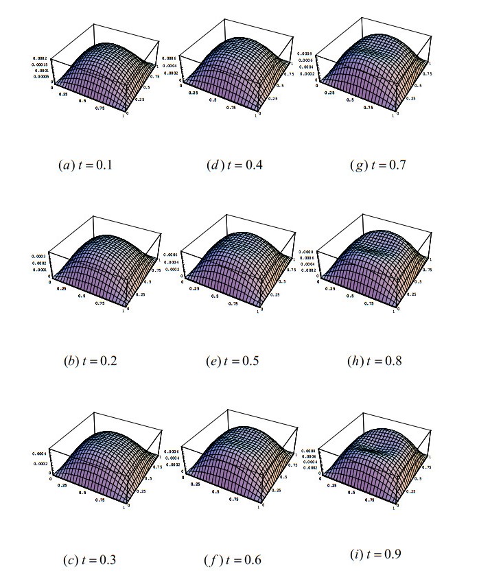
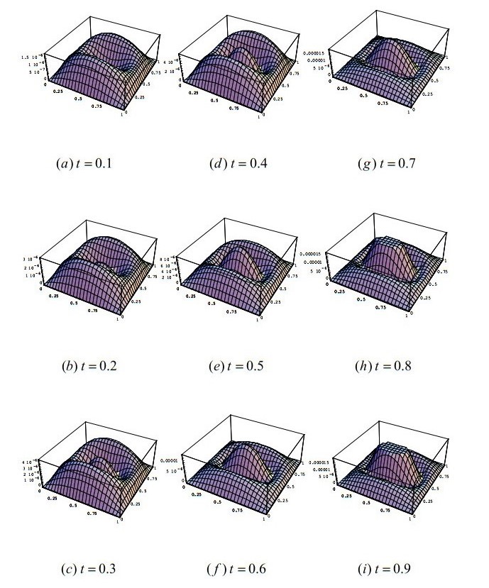
A novel method is presented for reproducing kernel of a 2D fractional diffusion equation. The exact solution is expressed as a series, which is then truncated to get an approximate solution. In addition, some techniques to improve existing methods are also proposed. The proposed approach is easy to implement. It is proved that both the approximate solution and its partial derivatives converge to their exact solutions. Numerical results demonstrate that the proposed approach is effective and can provide a high precision global approximate solution.
Citation: Siyu Tian, Boyu Liu, Wenyan Wang. A novel numerical scheme for reproducing kernel space of 2D fractional diffusion equations[J]. AIMS Mathematics, 2023, 8(12): 29058-29072. doi: 10.3934/math.20231488
A novel method is presented for reproducing kernel of a 2D fractional diffusion equation. The exact solution is expressed as a series, which is then truncated to get an approximate solution. In addition, some techniques to improve existing methods are also proposed. The proposed approach is easy to implement. It is proved that both the approximate solution and its partial derivatives converge to their exact solutions. Numerical results demonstrate that the proposed approach is effective and can provide a high precision global approximate solution.

| [1] |
K. B. Oldham, Fractional differential equations in electrochemistry, Adv. Eng. Softw., 41 (2010), 9–12. https://doi.org/10.1016/j.advengsoft.2008.12.012 doi: 10.1016/j.advengsoft.2008.12.012

|
| [2] |
Y. Z. Povstenko, Evolution of the initial box-signal for time-fractional diffusion-wave equation in a case of different spatial dimensions, Physica A, 389 (2010), 4696–4707. https://doi.org/10.1016/j.physa.2010.06.049 doi: 10.1016/j.physa.2010.06.049
|
| [3] |
C. Ming, F. Liu, L. Zheng, I. Turner, V. Anh, Analytical solutions of multi-term time fractional differential equations and application to unsteady flows of generalized viscoelastic fluid, Comput. Math. Appl., 72 (2016), 2084–2097. https://doi.org/10.1016/j.camwa.2016.08.012 doi: 10.1016/j.camwa.2016.08.012
|
| [4] |
S. Kumar, R. Kumar, C. Cattani, B. Samet, Chaotic behaviour of fractional predator-prey dynamical system, Chaos Soliton. Fract., 135 (2020), 109811. https://doi.org/10.1016/j.chaos.2020.109811 doi: 10.1016/j.chaos.2020.109811
|
| [5] |
S. Kumar, S. Ghosh, M. S. M. Lotayif, B. Samet, A model for describing the velocity of a particle in Brownian motion by Robotnov function based fractional operator, Alex. Eng. J., 59 (2020), 1435–1449. https://doi.org/10.1016/j.aej.2020.04.019 doi: 10.1016/j.aej.2020.04.019
|
| [6] |
S. T. Abdulazeez, M. Modanli, Solutions of fractional order pseudo-hyperbolic telegraph partial differential equations using finite difference method, Alex. Eng. J., 61 (2022), 12443–12451. https://doi.org/10.1016/j.aej.2022.06.027 doi: 10.1016/j.aej.2022.06.027
|
| [7] |
O. Nave, Modification of semi-analytical method applied system of ODE, Modern Applied Science, 14 (2020), 75–81. https://doi.org/10.5539/mas.v14n6p75 doi: 10.5539/mas.v14n6p75
|
| [8] |
W. M. Abd-Elhameed, Y. H. Youssri, New formulas of the high-order derivatives of fifth-kind Chebyshev polynomials: Spectral solution of the convection-diffusion equation, Numer. Meth. Part. D. E., 2021 (2021), 22756. https://doi.org/10.1002/num.22756 doi: 10.1002/num.22756
|
| [9] |
A. G. Atta, W. M. Abd-Elhameed, Y. H. Youssri, Shifted fifth-kind Chebyshev polynomials Galerkin-based procedure for treating fractional diffusion-wave equation, Int. J. Mod. Phys. C, 33 (2022), 2250102. https://doi.org/10.1142/S0129183122501029 doi: 10.1142/S0129183122501029
|
| [10] |
R. M. Hafez, Y. H. Youssri, Jacobi collocation scheme for variable-order fractional reaction-subdiffusion equation, Comp. Appl. Math., 37 (2018), 5315–5333. https://doi.org/10.1007/s40314-018-0633-3 doi: 10.1007/s40314-018-0633-3
|
| [11] |
Y. H. Youssri, A. G. Atta, Petrov-Galerkin Lucas polynomials procedure for the time-fractional diffusion equation, Contemp. Math., 4 (2023), 230–248. https://doi.org/10.37256/cm.4220232420 doi: 10.37256/cm.4220232420
|
| [12] |
P. K. Gupta, Approximate analytical solutions of fractional Benney-Lin equation by reduced differential transform method and the homotopy perturbation method, Comp. Math. Appl., 61 (2011), 2829–2842. https://doi.org/10.1016/j.camwa.2011.03.057 doi: 10.1016/j.camwa.2011.03.057
|
| [13] |
M. A. Attar, M. Roshani, K. Hosseinzadeh, D. D. Ganji, Analytical solution of fractional differential equations by Akbari-Ganji's method, Partial Differential Equations in Applied Mathematics, 6 (2022), 100450. https://doi.org/10.1016/j.padiff.2022.100450 doi: 10.1016/j.padiff.2022.100450
|
| [14] |
C. Bota, B. Caruntu, Analytical approximate solutions for quadratic Riccati differential equation of fractional order using the polynomial least squares method, Chaos Soliton. Fract., 102 (2017), 339–345. https://doi.org/10.1016/j.chaos.2017.05.002 doi: 10.1016/j.chaos.2017.05.002
|
| [15] | M. Moustafa, Y. H. Youssri, A. G. Atta, Explicit Chebyshev-Galerkin scheme for the time-fractional diffusion equation, in press. https://doi.org/10.1142/S0129183124500025 |
| [16] |
S. Djennadi, N. Shawagfeh, O. A. Arqub, A numerical algorithm in reproducing kernel-based approach for solving the inverse source problem of the time-space fractional diffusion equation, Partial Differential Equations in Applied Mathematics, 4 (2021), 100164. https://doi.org/10.1016/j.padiff.2021.100164 doi: 10.1016/j.padiff.2021.100164
|
| [17] |
W. Jiang, Y. Lin, Approximate solution of the fractional advection-dispersion equation, Comput. Phys. Commun., 181 (2010), 557–561. https://doi.org/10.1016/j.cpc.2009.11.004 doi: 10.1016/j.cpc.2009.11.004
|
| [18] |
R. Metzler, J. Klafter, Boundary value problems for fractional diffusion equations, Physica A, 278 (2000), 107–125. https://doi.org/10.1016/S0378-4371(99)00503-8 doi: 10.1016/S0378-4371(99)00503-8
|
| [19] | A. A. Kilbas, H. M. Srivastava, J. J. Trujillo, Theory and applications of fractional differential equations, Amsterdam: Elsevier, 2006. |
| [20] | I. Podlubny, Fractional differential equations, San Diego: Academic Press, 1999. |
| [21] |
W. Jiang, Z. Chen, Solving a system of linear Volterra integral equations using the new reproducing kernel method, Appl. Math. Comput., 219 (2013), 10225–10230. https://doi.org/10.1016/j.amc.2013.03.123 doi: 10.1016/j.amc.2013.03.123
|
| [22] |
X. Li, B. Wu, A kernel regression approach for identification of first order differential equations based on functional data, Appl. Math. Lett., 127 (2022), 107832. https://doi.org/10.1016/j.aml.2021.107832 doi: 10.1016/j.aml.2021.107832
|
| [23] |
F. Geng, X. Wu, Reproducing kernel functions based univariate spline interpolation, Appl. Math. Lett., 122 (2021), 107525. https://doi.org/10.1016/j.aml.2021.107525 doi: 10.1016/j.aml.2021.107525
|
| [24] |
M. G. Sakar, Iterative reproducing kernel Hilbert spaces method for Riccati differential equations, J. Comput. Appl. Math., 309 (2017), 163–174. https://doi.org/10.1016/j.cam.2016.06.029 doi: 10.1016/j.cam.2016.06.029
|
| [25] |
M. Cui, Z. Chen, The exact solution of nonlinear age-structured population model, Nonlinear Anal. Real, 8 (2007), 1096–1112. https://doi.org/10.1016/j.nonrwa.2006.06.004 doi: 10.1016/j.nonrwa.2006.06.004
|
| [26] |
J. Niu, Y. Jia, J. Sun, A new piecewise reproducing kernel function algorithm for solving nonlinear Hamiltonian systems, Appl. Math. Lett., 136 (2023), 108451. https://doi.org/10.1016/j.aml.2022.108451 doi: 10.1016/j.aml.2022.108451
|
| [27] |
W. Wang, M. Cui, B. Han, A new method for solving a class of singular two-point boundary value problems, Appl. Math. Comput., 206 (2008), 721–727. https://doi.org/10.1016/j.amc.2008.09.019 doi: 10.1016/j.amc.2008.09.019
|
| [28] |
X. Su, J. Yang, H. Yao, Shifted Legendre reproducing kernel Galerkin method for the quasilinear degenerate parabolic problem, Appl. Math. Lett., 135 (2023), 108416. https://doi.org/10.1016/j.aml.2022.108416 doi: 10.1016/j.aml.2022.108416
|
| [29] |
X. Li, B. Wu, Error estimation for the reproducing kernel method to solve linear boundary value problems, J. Comput. Appl. Math., 243 (2013), 10–15. https://doi.org/10.1016/j.cam.2012.11.002 doi: 10.1016/j.cam.2012.11.002
|
| [30] |
F. Geng, X. Wu, Reproducing kernel functions based univariate spline interpolation, Appl. Math. Lett., 122 (2021), 107525. https://doi.org/10.1016/j.aml.2021.107525 doi: 10.1016/j.aml.2021.107525
|
| [31] |
X. Li, B.Wu, Reproducing kernel functions-based meshless method for variable order fractional advection-diffusion-reaction equations, Alex. Eng. J., 59 (2020), 3181–3186. https://doi.org/10.1016/j.aej.2020.07.034 doi: 10.1016/j.aej.2020.07.034
|
| [32] |
G. Zheng, T. Wei, Spectral regularization method for a Cauchy problem of the time fractional advection-dispersion equation, J. Comput. Appl. Math., 233 (2010), 2631–2640. https://doi.org/10.1016/j.cam.2009.11.009 doi: 10.1016/j.cam.2009.11.009
|
| [33] |
O. Saldlr, M. G. Sakar, F. Erdogan, Numerical solution of time-fractional Kawahara equation using reproducing kernel method with error estimate, Comp. Appl. Math., 38 (2019), 198. https://doi.org/10.1007/s40314-019-0979-1 doi: 10.1007/s40314-019-0979-1
|
| [34] |
Y. Wang, M. Du, F. Tan, Z. Li, T. Nie, Using reproducing kernel for solving a class of fractional partial differential equation with non-classical conditions, Appl. Math. Comput., 219 (2013), 5918–5925. https://doi.org/10.1016/j.amc.2012.12.009 doi: 10.1016/j.amc.2012.12.009
|
| [35] |
W. Wang, M. Yamamoto, B. Han, Two-dimensional parabolic inverse source problem with final overdetermination in reproducing kernel space, Chin. Ann. Math. Ser. B, 35 (2014), 469–482. https://doi.org/10.1007/s11401-014-0831-2 doi: 10.1007/s11401-014-0831-2
|
| [36] |
W. Wang, B. Han, M. Yamamoto, Inverse heat problem of determining time-dependent source parameter in reproducing kernel space, Nonlinear Anal. Real, 14 (2013), 875–887. https://doi.org/10.1016/j.nonrwa.2012.08.009 doi: 10.1016/j.nonrwa.2012.08.009
|
| [37] | M. Cui, Y. Lin, Nonlinear numerical analysis in the reproducing kernel space, New York: Nova Science, 2009. |
| [38] |
M. Cui, F. Geng, A computational method for solving one-dimensional variable-coeffificient Burgers equation, Appl. Math. Comput., 188 (2007), 1389–1401. https://doi.org/10.1016/j.amc.2006.11.005 doi: 10.1016/j.amc.2006.11.005
|
Figures(2) / Tables(4)

Siyu Tian, Boyu Liu, Wenyan Wang. A novel numerical scheme for reproducing kernel space of 2D fractional diffusion equations[J]. AIMS Mathematics, 2023, 8(12): 29058-29072. doi: 10.3934/math.20231488


 DownLoad: