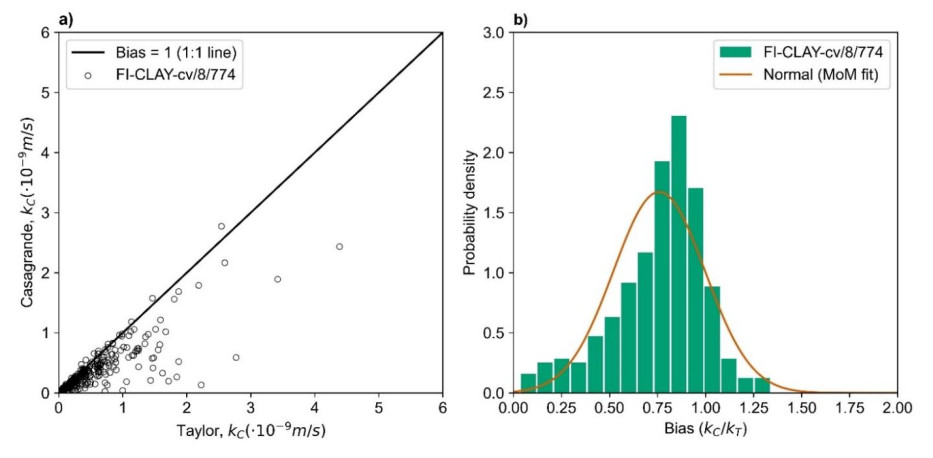
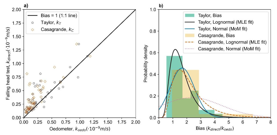
When constructing on clay and gyttja soils, low-carbon ground improvement methods such as preloading should be preferred over carbon-intensive solutions (e.g., piles or deep mixing with lime-cement binder). The design of preloading requires knowledge about the compressibility and consolidation properties of subsoil, but site-specific oedometer tests may be scarce or even lacking, especially in the early design phases. Hence, this paper presents two extensive databases based on oedometer tests performed on Finnish clay and gyttja soils, with a special emphasis on consolidation rate and creep properties. The FI-CLAY-oedo/14/282 database contains 282 oedometer test-specific data entries, such as initial hydraulic conductivity and maximum creep coefficient. The second database, FI-CLAY-cv/8/774, contains 774 load increment–specific data entries (e.g., coefficient of consolidation) from 232 oedometer tests. The analysis of these databases provided three main results: (ⅰ) statistics for bias factors, which quantify the differences between determination methods (log time vs. square root time method and oedometer vs. falling head test), (ⅱ) transformation models (and their transformation uncertainty) to predict creep coefficient from index or consolidation properties, and (ⅲ) typical value distributions for various consolidation rate and creep properties, in a form of histograms and fitted lognormal distributions. All the results are given with statistical information, which allows their straightforward utilization as input data for probabilistic assessment (reliability-based design). It is concluded that the consolidation properties of clay and gyttja soils are indeed characterized by significant uncertainty. Hence, such results are recommended to be used as existing (prior) knowledge when determining design parameters, either by supporting engineering judgement or via a more systematic framework such as Bayesian statistics.
Citation: Monica S Löfman, Leena Korkiala-Tanttu. Consolidation properties of clay and gyttja soils: A database study[J]. AIMS Geosciences, 2025, 11(2): 343-369. doi: 10.3934/geosci.2025015
When constructing on clay and gyttja soils, low-carbon ground improvement methods such as preloading should be preferred over carbon-intensive solutions (e.g., piles or deep mixing with lime-cement binder). The design of preloading requires knowledge about the compressibility and consolidation properties of subsoil, but site-specific oedometer tests may be scarce or even lacking, especially in the early design phases. Hence, this paper presents two extensive databases based on oedometer tests performed on Finnish clay and gyttja soils, with a special emphasis on consolidation rate and creep properties. The FI-CLAY-oedo/14/282 database contains 282 oedometer test-specific data entries, such as initial hydraulic conductivity and maximum creep coefficient. The second database, FI-CLAY-cv/8/774, contains 774 load increment–specific data entries (e.g., coefficient of consolidation) from 232 oedometer tests. The analysis of these databases provided three main results: (ⅰ) statistics for bias factors, which quantify the differences between determination methods (log time vs. square root time method and oedometer vs. falling head test), (ⅱ) transformation models (and their transformation uncertainty) to predict creep coefficient from index or consolidation properties, and (ⅲ) typical value distributions for various consolidation rate and creep properties, in a form of histograms and fitted lognormal distributions. All the results are given with statistical information, which allows their straightforward utilization as input data for probabilistic assessment (reliability-based design). It is concluded that the consolidation properties of clay and gyttja soils are indeed characterized by significant uncertainty. Hence, such results are recommended to be used as existing (prior) knowledge when determining design parameters, either by supporting engineering judgement or via a more systematic framework such as Bayesian statistics.

| [1] | Perttu O, Vicente S, Löfman M, et al. (2024) Carbon management in geotechnical engineering solutions, Geotechnical Engineering Challenges to Meet Current and Emerging Needs of Society, CRC Press, 3228–3232. |
| [2] | Kivi E (2022) Pohjanvahvistusmenetelmät Suomessa—Käyttömäärät ja hiilijalanjälki. Espoo: Aalto University. Available from: https://aaltodoc.aalto.fi/items/0a309556-72a4-468b-b089-cd6da2ec962a. |
| [3] | Lee IK, White W, Ingles OG (1983) Geotechnical Engineering, Boston: Pitman. |
| [4] | Leroueil S, Magnan J-P, Tavenas F (1990) Embankments on Soft Clay, Chichester: Ellis Horwood. |
| [5] | Gardemeister R (1975) On engineering-geological properties of fine-grained sediments in Finland. 91. |
| [6] |
Löfman MS, Korkiala-Tanttu LK (2022) Transformation models for the compressibility properties of Finnish clays using a multivariate database. Georisk Assess Manage Risk Eng Syst Geohazards 16: 330–346. https://doi.org/10.1080/17499518.2020.1864410 doi: 10.1080/17499518.2020.1864410

|
| [7] |
D'Ignazio M, Phoon KK, Tan SA, et al. (2016) Correlations for undrained shear strength of Finnish soft clays. Can Geotech J 53: 1628–1645. https://doi.org/10.1139/cgj-2016-0037 doi: 10.1139/cgj-2016-0037
|
| [8] | Baecher GB (2019) Putting Numbers on Geotechnical Judgment. Companion whitepaper to the 27th Buchanan Lecture, Texas A & M University. Available from: https://www.researchgate.net/publication/338801782_Baecher_2019_-_Putting_Numbers_on_Geotechnical_Judgment_27th_Buchanan_Lecture. |
| [9] |
Cao Z, Wang Y, Li D (2016) Quantification of prior knowledge in geotechnical site characterization. Eng Geol 203: 107–116. https://doi.org/10.1016/j.enggeo.2015.08.018 doi: 10.1016/j.enggeo.2015.08.018
|
| [10] |
Wang Y, Cao Z, Li D (2016) Bayesian perspective on geotechnical variability and site characterization. Eng Geol 203: 117–125. https://doi.org/10.1016/j.enggeo.2015.08.017 doi: 10.1016/j.enggeo.2015.08.017
|
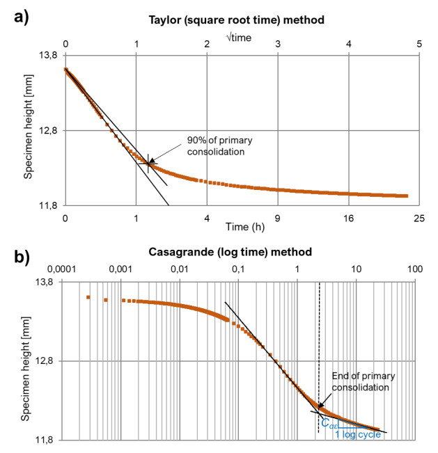
| [11] | Taylor DW (1948) Fundamentals of Soil Mechanics, New York, John Wiley & Sons Inc. |
| [12] | Casagrande A (1936) The determination of preconsolidation load and its practical significance. Proc 1st Int Conf Soil Mech. |
| [13] | Buisman A (1936) Results of Long Duration Settlement Tests. Int Conf Soil Mech Found Eng, 103–106. |
| [14] | Mesri G, Choi YK (1985) The uniquenes of the end-of-primary (EOP) void ratio-effective sress relationship. 587–590. |
| [15] | Larsson R (1986) Consolidation of soft soils, Linköping. |
| [16] |
Mesri G, Castro A (1987) C α/C c concept and K 0 during secondary compression. J Geotech Eng 113: 230–247. https://doi.org/10.1061/(ASCE)0733-9410(1987)113:3(230) doi: 10.1061/(ASCE)0733-9410(1987)113:3(230)
|
| [17] | Mataić I (2016) On structure and rate dependence of Perniö clay. |
| [18] | Suhonen K (2010) Creep of Soft Clay. Master thesis, Aalto University. 103. Available from: https://aaltodoc.aalto.fi/server/api/core/bitstreams/05a2a28b-aadd-4878-aa25-62a179ee52be/content. |
| [19] | Korhonen KH, Gardemeister R, Tammirinne M (1974) Geotekninen maaluokitus. Geotekniikan laboratorio, tiedonanto 14. Otaniemi, Espoo. Available from: https://publications.vtt.fi/julkaisut/muut/1970s/geotekniikan_tiedonanto_14.pdf. |
| [20] | Koskinen M (2014) Plastic Anisotropy and Destructuration of Soft Finnish Clays. Espoo: Aalto University. |
| [21] |
Phoon K-K, Kulhawy FH (1999) Characterization of geotechnical variability. Can Geotech J 36: 612–624. https://doi.org/10.1139/t99-038 doi: 10.1139/t99-038
|
| [22] |
Ching J, Phoon K-K (2014) Transformations and correlations among some clay parameters—The global database. Can Geotech J 51: 663–685. https://doi.org/10.1139/cgj-2013-0262 doi: 10.1139/cgj-2013-0262
|
| [23] | Pedregosa F, Varoquaux G, Gramfort A, et al. (2011) Scikit-learn: Machine Learning in Python. J Mach Learn Res 12: 2825–2830. |
| [24] | Ang AHS, Tang WH (2006) Probability Concepts in Engineering: Emphasis on Applications to Civil and Environmental Engineering. Wiley, 432. |
| [25] |
Berilgen SA, Berilgen MM, Ozaydin IK (2006) Compression and permeability relationships in high water content clays. Appl Clay Sci 31: 249–261. https://doi.org/10.1016/j.clay.2005.08.002 doi: 10.1016/j.clay.2005.08.002
|
| [26] |
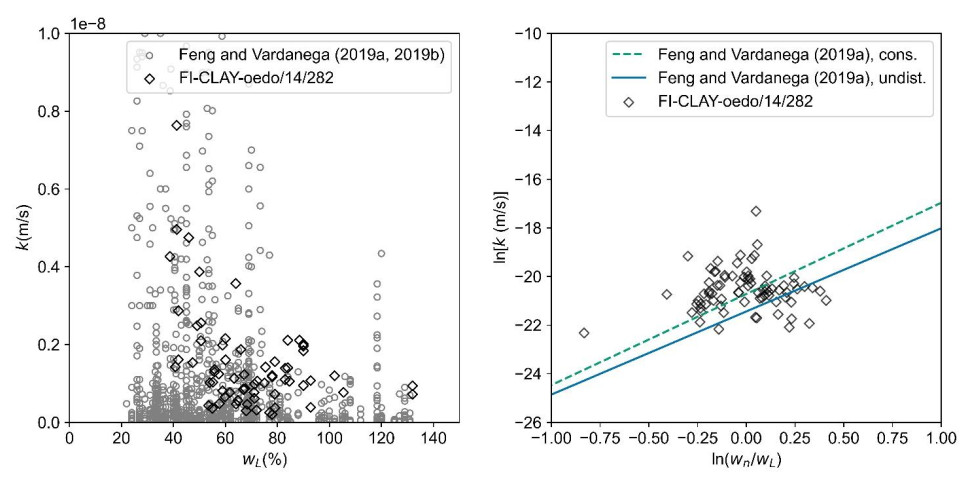
Feng S, Vardanega PJ (2019) Correlation of the hydraulic conductivity of fine-grained soils with water content ratio using a database. Environ Geotech 6: 253–268. https://doi.org/10.1680/jenge.18.00166 doi: 10.1680/jenge.18.00166
|
| [27] |
Feng S, Vardanega PJ (2019) A database of saturated hydraulic conductivity of fine-grained soils: probability density functions. Georisk Assess Manage Risk Eng Syst Geohazards 13: 255–261. https://doi.org/10.1080/17499518.2019.1652919 doi: 10.1080/17499518.2019.1652919
|
| [28] | Andersen JD (2012) Prediction of compression ratio for clays and organic soils. Proceedings of the 16th Nordic Geotechnical Meeting, Copenhagen, 1: 303–310. |
| [29] |
Phoon K-K, Tang C (2019) Characterisation of geotechnical model uncertainty. Georisk Assess Manage Risk Eng Syst Geohazards 13: 101–130. https://doi.org/10.1080/17499518.2019.1585545 doi: 10.1080/17499518.2019.1585545
|
| [30] | Ching J, Noorzad A (2021) Statistics for transformation uncertainties. State-of-the-art review of inherent variability and uncertainty in geotechnical properties and models, 171–180. |
| [31] | Uzielli M, Lacasse S, Nadim F, et al. (2006) Soil variability analysis for geotechnical practice. Charact Eng Prop Natural Soils 3: 1653–1752. |
| [32] | Löfman MS, Korkiala-Tanttu LK (2021) Inherent variability of geotechnical properties for Finnish clay soils. 18th International Probabilistic Workshop. IPW 2021. Lecture Notes in Civil Engineering, Springer, Cham. https://doi.org/10.1007/978-3-030-73616-3_32 |
| [33] |
Phoon K-K (2017) Role of reliability calculations in geotechnical design. Georisk Assess Manage Risk Eng Syst Geohazards 11: 4–21. https://doi.org/10.1080/17499518.2016.1265653 doi: 10.1080/17499518.2016.1265653
|
| [34] |
Ching J, Phoon K-K, Wu C-T (2022) Data-centric quasi-site-specific prediction for compressibility of clays. Can Geotech J 59: 2033–2049. https://doi.org/10.1139/cgj-2021-0658 doi: 10.1139/cgj-2021-0658
|
| [35] |
Phoon K-K, Zhang W (2023) Future of machine learning in geotechnics. Georisk Assess Manage Risk Eng Syst Geohazards 17: 7–22. https://doi.org/10.1080/17499518.2022.2087884 doi: 10.1080/17499518.2022.2087884
|
| [36] |
Zhang W, Li H, Li Y, et al. (2021) Application of deep learning algorithms in geotechnical engineering: a short critical review. Artif Intell Rev 54: 5633–5673. https://doi.org/10.1007/s10462-021-09967-1 doi: 10.1007/s10462-021-09967-1
|
 geosci-11-02-015-s001.xlsx geosci-11-02-015-s001.xlsx |
 |
| geosci-11-02-015-s002.xlsx |
|
Figures(22) / Tables(6)

Monica S Löfman, Leena Korkiala-Tanttu. Consolidation properties of clay and gyttja soils: A database study[J]. AIMS Geosciences, 2025, 11(2): 343-369. doi: 10.3934/geosci.2025015


 DownLoad: