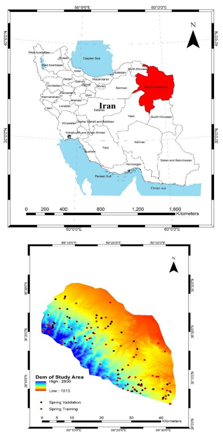
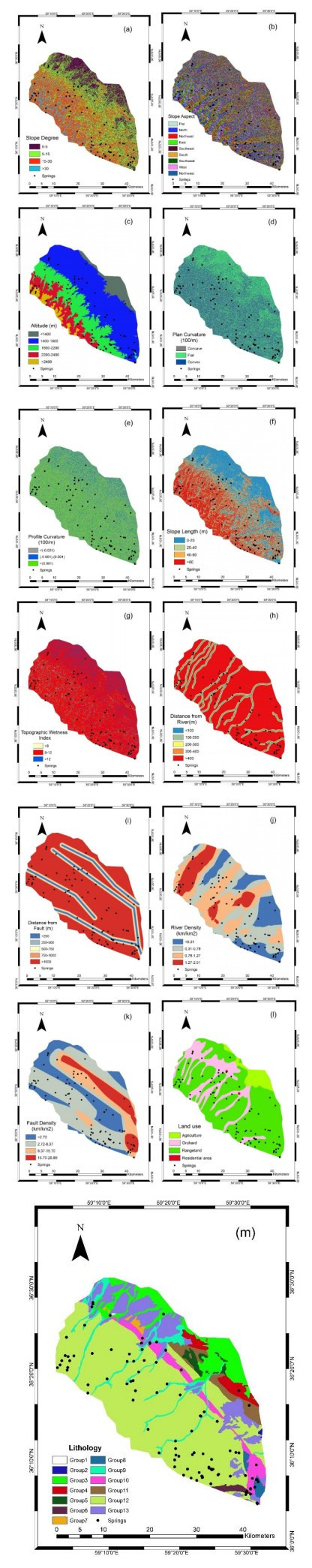
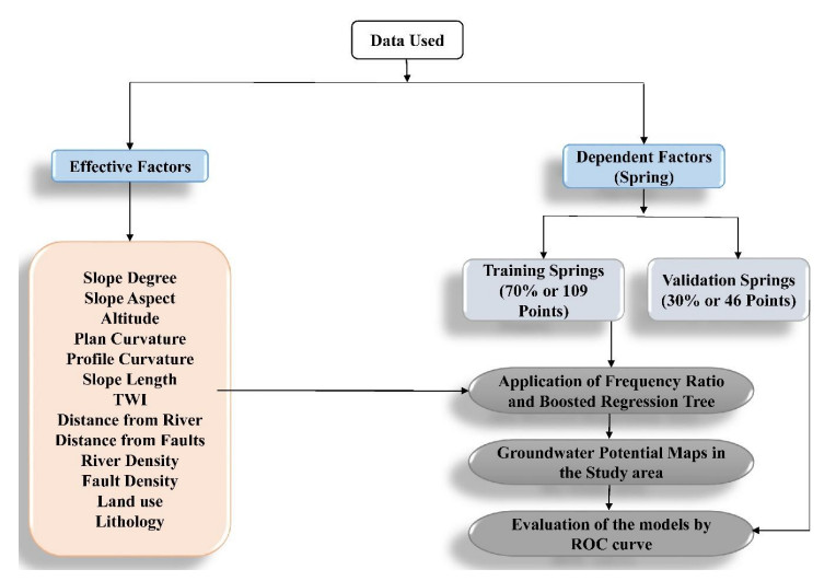
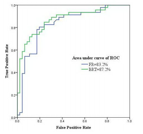
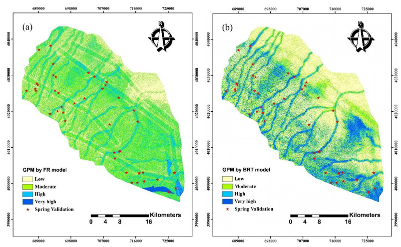
This study intends to investigate the performance of boosted regression tree (BRT) and frequency ratio (FR) models in groundwater potential mapping. For this purpose, location of the springs was determined in the western parts of the Mashhad Plain using national reports and field surveys. In addition, thirteen groundwater conditioning factors were prepared and mapped for the modelling process. Those factor maps are: slope degree, slope aspect, altitude, plan curvature, profile curvature, slope length, topographic wetness index, distance from faults, distance from rivers, river density, fault density, land use, and lithology. Then, frequency ratio and boosted regression tree models were applied and groundwater potential maps (GPMs) were produced. In the last step, validation of the models was carried out implementing receiver operating characteristics (ROC) curve. According to the results, BRT had area under curve of ROC (AUC-ROC) of 87.2%, while it was seen that FR had AUC-ROC of 83.2% that implies acceptable operation of the models. According to the results of this study, topographic wetness index was the most important factor, followed by altitude, and distance from rivers. On the other hand, aspect, and plan curvature were seen to be the least important factors. The methodology implemented in this study could be used for other basins with similar conditions to cope with water resources problem.
Citation: Seyed Mohsen Mousavi, Ali Golkarian, Seyed Amir Naghibi, Bahareh Kalantar, Biswajeet Pradhan. GIS-based Groundwater Spring Potential Mapping Using Data Mining Boosted Regression Tree and Probabilistic Frequency Ratio Models in Iran[J]. AIMS Geosciences, 2017, 3(1): 91-115. doi: 10.3934/geosci.2017.1.91
This study intends to investigate the performance of boosted regression tree (BRT) and frequency ratio (FR) models in groundwater potential mapping. For this purpose, location of the springs was determined in the western parts of the Mashhad Plain using national reports and field surveys. In addition, thirteen groundwater conditioning factors were prepared and mapped for the modelling process. Those factor maps are: slope degree, slope aspect, altitude, plan curvature, profile curvature, slope length, topographic wetness index, distance from faults, distance from rivers, river density, fault density, land use, and lithology. Then, frequency ratio and boosted regression tree models were applied and groundwater potential maps (GPMs) were produced. In the last step, validation of the models was carried out implementing receiver operating characteristics (ROC) curve. According to the results, BRT had area under curve of ROC (AUC-ROC) of 87.2%, while it was seen that FR had AUC-ROC of 83.2% that implies acceptable operation of the models. According to the results of this study, topographic wetness index was the most important factor, followed by altitude, and distance from rivers. On the other hand, aspect, and plan curvature were seen to be the least important factors. The methodology implemented in this study could be used for other basins with similar conditions to cope with water resources problem.

| [1] | Altenburger R, Ait-Aissa S, Antczak P, et al. (2015) Future water quality monitoring—adapting tools to deal with mixtures of pollutants in water resource management. Sci Total Environ 512: 540-551. |
| [2] | Chezgi J, Pourghasemi HR, Naghibi SA, et al. (2015) Assessment of a spatial multi-criteria evaluation to site selection underground dams in the Alborz Province, Iran. Geocarto Int 31: 628-646. |
| [3] | Oh HJ, Kim YS, Choi JK, et al. (2011) GIS mapping of regional probabilistic groundwater potential in the area of Pohang City, Korea. J Hydrol 399: 158-172. |
| [4] | Nampak H, Pradhan B, Manap MA (2014) Application of GIS based data driven evidential belief function model to predict groundwater potential zonation. J Hydrol 513: 283-300. |
| [5] | Tweed SO, Leblanc M, Webb JA, et al. (2007) Remote sensing and GIS for mapping groundwater recharge and discharge areas in salinity prone catchments, southeastern Australia. Hydrogeol J 15: 75-96. |
| [6] | Ozdemir A (2011a) Using a binary logistic regression method and GIS for evaluating and mapping the groundwater spring potential in the Sultan Mountains (Aksehir, Turkey). J Hydrol 405: 123-136. |
| [7] | Ozdemir A (2011b) GIS-based groundwater spring potential mapping in the Sultan Mountains (Konya, Turkey) using frequency ratio, weights of evidence and logistic regression methods and their comparison. J Hydrol 411: 290-308. |
| [8] | Manap MA, Nampak H, Pradhan B, et al. (2014) Application of probabilistic-based frequency ratio model in groundwater potential mapping using remote sensing data and GIS. Arabian J Geosci 7: 711-724. |
| [9] | Pourtaghi ZS and Pourghasemi HR (2014) GIS-based groundwater spring potential assessment and mapping in the Birjand Township, southern Khorasan Province, Iran. Hydrogeology J 22:643-662. |
| [10] | Naghibi SA, Pourghasemi HR, Pourtaghi ZS, et al. (2015) Groundwater qanat potential mapping using frequency ratio and Shannon's entropy models in the Moghan watershed, Iran. Earth Sci Inform 8: 171-186. |
| [11] | Pourghasemi HR, Beheshtirad M (2015) Assessment of a data-driven evidential belief function model and GIS for groundwater potential mapping in the Koohrang Watershed, Iran. Geocarto Int 30: 662-685. |
| [12] | Naghibi SA, Pourghasemi HR (2015) A comparative assessment between three machine learning models and their performance comparison by bivariate and multivariate statistical methods in groundwater potential mapping. Water Res Manage 29: 5217-5236. |
| [13] | Al-Abadi A, M Pradhan B, Shahid S (2015) Prediction of groundwater flowing well zone at An-Najif Province, central Iraq using evidential belief functions model and GIS. Environ Monit Assess 188:549. |
| [14] | Naghibi SA, Pourghasemi HR, Dixon B (2016) GIS-based groundwater potential mapping using boosted regression tree, classification and regression tree, and random forest machine learning models in Iran. Environ Monit Assess 188: 1-27. |
| [15] | Naghibi S A, Dashtpagerdi MM (2016) Evaluation of four supervised learning methods for groundwater spring potential mapping in Khalkhal region (Iran) using GIS-based features. Hydrogeol J 1-21. |
| [16] | Zabihi M, Pourghasemi, HR, Pourtaghi ZS, et al. (2016) GIS-based multivariate adaptive regression spline and random forest models for groundwater potential mapping in Iran. Environ Earth Sci 75: 1-19. |
| [17] | Naghibi SA, Pourghasemi HR. , Abbaspour K (2017). A comparison between ten advanced and soft computing models for groundwater qanat potential assessment in Iran using R and GIS. Theoretical and Applied Climatology. |
| [18] | Mennis J and Guo D (2009) Spatial data mining and geographic knowledge discovery—an introduction. Comput Environ Urban Syst 33:403-408. |
| [19] | Tien Bui D, Le K-T, Nguyen V (2016a) Tropical forest fire susceptibility mapping at the Cat Ba National Park Area, Hai Phong City, Vietnam, using GIS-based Kernel logistic regression. Remote Sens 8: 347. |
| [20] | Pacheco, Fernando, Ana Alencoão (2002) "Occurrence of springs in massifs of crystalline rocks, northern Portugal." Hydrogeol J 10.2: 239-253. |
| [21] | Pacheco FAL and Vander Weijden CH (2014). Modeling rock weathering in small watersheds. J Hydrol 513C 13-27. |
| [22] | Iranian Department of Water Resources Management (2014) weather and climate report, Tehran province. Available from: http://www.thrw.ir/. |
| [23] | Dehnavi A, Aghdam IN, Pradhan B, et al. (2015) A new hybrid model using step-wise weight assessment ratio analysis (SWARA) technique and adaptive neuro-fuzzy inference system (ANFIS) for regional landslide hazard assessment in Iran. Catena 135: 122-148. |
| [24] | Conforti M, Pascale S, Robustelli G, et al. (2014) Evaluation of prediction capability of the artificial neural networks for mapping landslide susceptibility in the Turbolo River catchment (northern Calabria, Italy). Catena 113: 236-250. |
| [25] | Oh H-J and Pradhan B (2011) Application of a neuro-fuzzy model to landslide-susceptibility mapping for shallow landslides in a tropical hilly area. Comput Geosci 37: 1264-1276. |
| [26] | Wilson JP and Gallant JG (2000) Terrain Analysis Principles and Applications. John Wiley and Sons, Inc. , New-York, 479. |
| [27] | Moore ID and Burch GJ (1986) Sediment Transport Capacity of Sheet and Rill Flow: Application of Unit Stream Power Theory. Water Resour Res 22: 1350-1360. |
| [28] | Pourghasemi H, Pradhan B, Gokceoglu C, et al. (2013) A comparative assessment of prediction capabilities of Dempster-Shafer and weights-of-evidence models in landslide susceptibility mapping using GIS. Geomatics Nat Hazards Risk 4: 93-118. |
| [29] | Moore ID, Grayson RB, Ladson AR (1991) Digital terrain modelling: A review of hydrological, geomorphological, and biological applications. Hydrol Process 5: 3-30. |
| [30] | Ayalew L and Yamagishi H (2005) The application of GIS-based logistic regression for land-slide susceptibility mapping in the Kakuda-Yahiko Mountains, Central Japan. Geomorphol 65: 15-31. |
| [31] | Pradhan B, Abokharima MH, Jebur MN, et al. (2014) Land subsidence susceptibility mapping at Kinta Valley (Malaysia) using the evidential belief function model in GIS. Nat Hazards. |
| [32] | Iranian forest, rangeland and watershed management organization. 2014. Available from: http://www.frw.org.ir/00/En/default.aspx. |
| [33] | Geology Survey of Iran (GSI) (1997) Geology map of the Chaharmahal-e-Bakhtiari Province. http://www.gsi.ir/Main/Lang_en/index.html.AccessedSeptember2000. |
| [34] | Dormann CF, Elith J, Bacher S, et al. (2013) Collinearity: a review of methods to deal with it and a simula-tion study evaluating their performance. Ecogr 36: 27-46 |
| [35] | Hair JF, Black WC, Babin BJ, et al. (2009) Multivariate data analysis. Prentice Hall, New York. |
| [36] | Keith TZ (2006) Multiple regressions and beyond. Pearson, Boston |
| [37] | Lee S and Talib JA (2005) Probabilistic landslide susceptibility and factor effect analysis. Environ Geol 47: 982-990 |
| [38] | Yilmaz I (2007) GIS based susceptibility mapping of karst depression in gypsum: a case study from Sivas basin (Turkey). Eng Geol 90: 89-103 |
| [39] | Bonham-Carter G (1994) Geographic information systems for geoscientists modelling with GIS. Pergamon. |
| [40] | Lee S and Pradhan B (2006) Probabilistic landslide hazards and riskmapping on Penang Island, Malaysia. Earth Sys Sci 115: 661-667 |
| [41] | Lombardo L, Cama M, Conoscenti C, et al. (2015) Binary logistic regression versus stochastic gradient boosted decision trees in assessing landslide susceptibility for multiple-occurring landslide events: application to the 2009 storm event in Messina (Sicily, southern Italy). Nat Hazards 79: 1621-1648. |
| [42] | Abeare SM (2009) Comparisons of boosted regression tree, glm and gam performance in the standardization of yellowfin tuna catch-rate data from the gulf of mexico lonline fishery. |
| [43] | Friedman J (2001) Greedy boosting approximation: a gradient boosting machine. Ann Stat 29: 1189-1232. |
| [44] | Schapire RE (2003) The boosting approach to machine learning: an overview. Nonlinear Est Class 171: 149-171. |
| [45] | Sutton CD (2005) 11-Classification and Regression Trees, Bagging, and Boosting. Handbook of statistics 24: 303-329 |
| [46] | Kuhn M, Wing J, Weston S, et al. (2015) Package "caret". Available from: http://caret.r-forge.r-project.org. |
| [47] | Elith J, Leathwick JR, Hastie T (2008) A working guide to boosted regression trees. J Animal Ecol 77: 802-813 |
| [48] | Leathwick JR, Elith J, Francis MP, et al. (2006). Variation in demersal fish species richness in the oceans surrounding New Zealand: An analysis using boosted regression trees. Mar Ecol Prog Ser 321: 267-281. |
| [49] | Schillaci C, Lombardo L, Saia S, et al. (2017) Modelling the topsoil carbon stock of agricultural lands with the Stochastic Gradient Treeboost in a semi-arid Mediterranean region. Geoderma 286: 35-45. |
| [50] | R Development Core Team (2006) R: A Language and Environment for Statistical Computing, R Foundation for Statistical Computing, Vienna, Austria. ISBN 3-900051-07-0. Available from: http://www.R-project.org |
| [51] | Ridgeway G (2015) Package "gbm. " |
| [52] | Guzzetti F, Reichenbach P, Ardizzone F, et al. (2006) Estimating the quality of landslide susceptibility models. Geomorphol 81: 166-184 |
| [53] | Umar Z, Pradhan B, Ahmad A, et al. (2014) Earthquake induced landslide susceptibility mapping using an integrated ensemble frequency ratio and logistic regression models in West Sumatera Province, Indonesia. Catena 118: 124-135 |
| [54] | Swets JA (1988) Measuring the accuracy of diagnostic systems. Sci 240: 1285-1293 |
| [55] | Negnevitsky M (2005) Artificial Intelligence: a guide to intelligent systems. Inf & Comput Sci 48: 284-300. |
| [56] | Frattini P, Crosta G, Carrara A (2010). Techniques for evaluating the performance of landslide susceptibility models. Eng Geol 111: 62-72. |
| [57] | Lombardo L, Cama M, Maerker M., et al. (2014). A test of transferability for landslides susceptibility models under extreme climatic events: Application to the Messina 2009 disaster. Natural Hazards 74: 1951-1989. |
| [58] | Heckman T, Gegg K, Gegg A, et al. (2014) Sample size matters: investigating the effect of sample size on a logistic regression susceptibility model for debris flow. Nat. Hazards Earth Syst. Sci 14: 259-278. |
| [59] | Youssef AM, Pourghasemi HR, Pourtaghi ZS, et al. (2015) Landslide susceptibility mapping using random forest, boosted regression tree, classification and regression tree, and general linear models and comparison of their performance at Wadi Tayyah Basin, Asir Region, Saudi Arabia. Landslides 1-18 |
| [60] | Carty DM (2011) An analysis of boosted regression trees to predict the strength properties of wood composites. Arch Oral Biol 60: 45-54. |
Figures(6) / Tables(5)

Seyed Mohsen Mousavi, Ali Golkarian, Seyed Amir Naghibi, Bahareh Kalantar, Biswajeet Pradhan. GIS-based Groundwater Spring Potential Mapping Using Data Mining Boosted Regression Tree and Probabilistic Frequency Ratio Models in Iran[J]. AIMS Geosciences, 2017, 3(1): 91-115. doi: 10.3934/geosci.2017.1.91


 DownLoad: