The alternating direction implicit difference scheme and extrapolation method for a class of three dimensional hyperbolic equations with constant coefficients

Zhaoxiang Zhang; Xuehua Yang; Song Wang; Zhaoxiang Zhang; Xuehua Yang; Song Wang

doi:10.3934/era.2025148

Electronic Research Archive

2025, Volume 33, Issue 5: 3348-3377. doi: 10.3934/era.2025148

Previous Article Next Article

Research article Special Issues

The alternating direction implicit difference scheme and extrapolation method for a class of three dimensional hyperbolic equations with constant coefficients

1.
School of Science, Hunan University of Technology, Zhuzhou 412007, China
2.
School of Electrical Engineering, Computing and Mathematical Sciences, Curtin University, GPO Box U1987 Perth, WA 6845, Australia

Received: 25 March 2025 Revised: 07 May 2025 Accepted: 14 May 2025 Published: 29 May 2025

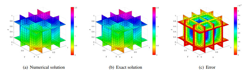
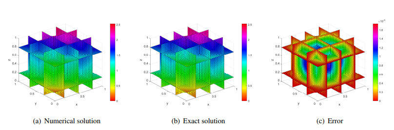
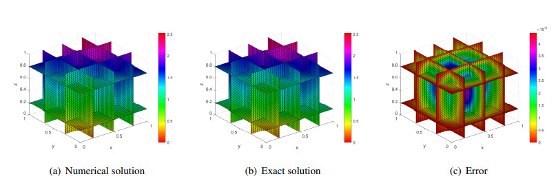
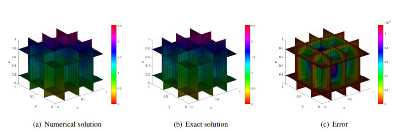
This paper conducts a study on the alternating direction implicit (ADI) difference schemes for a class of three dimensional hyperbolic equations with constant coefficients. The central difference methods are employed in the temporal and spatial direction. The solvability, stability, and convergence of the proposed ADI schemes are proven. Moreover, the Richardson extrapolation method is established to enhance the accuracy of the algorithm. Numerical examples are presented for the errors and convergence orders of the established ADI schemes and extrapolation schemes. By comparing the results of numerical examples, it can be concluded that the proposed Richardson extrapolation method can effectively improve the accuracy of the numerical solutions and reduce the errors.
- constant coefficient hyperbolic equation,
- three dimensional,
- finite difference method,
- ADI scheme,
- richardson extrapolation
Citation: Zhaoxiang Zhang, Xuehua Yang, Song Wang. The alternating direction implicit difference scheme and extrapolation method for a class of three dimensional hyperbolic equations with constant coefficients[J]. Electronic Research Archive, 2025, 33(5): 3348-3377. doi: 10.3934/era.2025148

Related Papers:

Abstract

This paper conducts a study on the alternating direction implicit (ADI) difference schemes for a class of three dimensional hyperbolic equations with constant coefficients. The central difference methods are employed in the temporal and spatial direction. The solvability, stability, and convergence of the proposed ADI schemes are proven. Moreover, the Richardson extrapolation method is established to enhance the accuracy of the algorithm. Numerical examples are presented for the errors and convergence orders of the established ADI schemes and extrapolation schemes. By comparing the results of numerical examples, it can be concluded that the proposed Richardson extrapolation method can effectively improve the accuracy of the numerical solutions and reduce the errors.

References

[1]	M. Dehghan, A. Ghesmati, Combination of meshless local weak and strong (MLWS) forms to solve the two dimensional hyperbolic telegraph equation, Eng. Anal. Bound. Elem., 32 (2010), 324–336. https://doi.org/10.1016/j.enganabound.2009.10.010 doi: 10.1016/j.enganabound.2009.10.010
[2]	A. Saadatmandi, M. Dehghan, Numerical solution of hyperbolic telegraph equation using the Chebyshev tau method, Numer. Methods Partial Differ. Equations, 26 (2010), 239–252. https://doi.org/10.1002/num.20442 doi: 10.1002/num.20442
[3]	R. Jiwari, S. Pandit, R. Mittal, A differential quadrature algorithm to solve the two dimensional linear hyperbolic telegraph equation with Dirichlet and Neumann boundary conditions, Appl. Math. Comput., 218 (2012), 7279–7294. https://doi.org/10.1016/j.amc.2012.01.006 doi: 10.1016/j.amc.2012.01.006
[4]	K. Zhukovsky, Operational approach and solutions of hyperbolic heat conduction equations, Axioms, 5 (2016), 28. https://doi.org/10.3390/axioms5040028 doi: 10.3390/axioms5040028
[5]	M. S. Yudin, Inversion effects on wind and surface pressure in atmospheric front propagation simulation with a hyperbolic model, Carpath. J. Earth. Env., 96 (2017), e012002. https://doi.org/10.1088/1755-1315/96/1/012002 doi: 10.1088/1755-1315/96/1/012002
[6]	T. Hillen, K. Hadeler, Hyperbolic systems and transport equations in mathematical biology, Carpath. J. Earth. Env., (2005), 257–279. https://doi.org/10.1007/3-540-27907-5_11 doi: 10.1007/3-540-27907-5_11
[7]	W. Alt, Inversion effects on wind and surface pressure in atmospheric front propagation simulation with a hyperbolic model, Carpath. J. Earth. Env., (2003), 431–461. https://doi.org/10.1088/1755-1315/96/1/012002 doi: 10.1088/1755-1315/96/1/012002
[8]	K. K. Sharma, P. Singh, Hyperbolic partial differential-difference equation in the mathematical modeling of neuronal firing and its numerical solution, Carpath. J. Earth. Env., 201 (2008), 229–238. https://doi.org/10.1016/j.amc.2007.12.051 doi: 10.1016/j.amc.2007.12.051
[9]	K. Hadeler, K. Dietz, Nonlinear hyperbolic partial differential equations for the dynamics of parasite populations, Hyperbolic Part. Differ. Equations, (1983), 415–430. https://doi.org/10.1016/B978-0-08-030254-6.50016-1 doi: 10.1016/B978-0-08-030254-6.50016-1
[10]	I. Fedotov, M. Shatalov, J. Marais, Hyperbolic and pseudo-hyperbolic equations in the theory of vibration, Acta. Mech., 227 (2016), 3315–3324. https://doi.org/10.1007/s00707-015-1537-6 doi: 10.1007/s00707-015-1537-6
[11]	G. Paul, Huygens' Principle and Hyperbolic Equations, Academic Press, 2014.
[12]	S. Alinhac, Blowup for Nonlinear Hyperbolic Equations, Springer Science & Business Media, 2013.
[13]	M. Dehghan, A. Ghesmati, Solution of the second-order one-dimensional hyperbolic telegraph equation by using the dual reciprocity boundary integral equation (DRBIE) method, Eng. Anal. Bound. Elem., 34 (2010), 51–59. https://doi.org/10.1016/j.enganabound.2009.07.002 doi: 10.1016/j.enganabound.2009.07.002
[14]	A. Häck, Kinetic and Hyperbolic Equations with Applications to Engineering Processes, Ph.D thesis, Dissertation, RWTH Aachen University, 2017.
[15]	O. A. Ladyzhenskaya, The Mixed Problem for a Hyperbolic Equation, Gostekhizdat, MoscowX, 1953.
[16]	R. Sakamoto, Hyperbolic Boundary Value Problems, Cup Archive, 1982.
[17]	V. M. Gordienko, Dissipativity of boundary condition in a mixed problem for the three-dimensional wave equation, Sib. Electron. Math. Rep., 10 (2013), 311–323. https://www.mathnet.ru/eng/semr/v10/p311
[18]	A. N. Malyshev, A mixed problem for a second-order hyperbolic equation with a complex first-order boundary condition, Sibirskii Matematicheskii Zhurnal, 24 (1983), 102–121. https://doi.org/10.1007/BF00970317 doi: 10.1007/BF00970317
[19]	K. Liu, Z. He, H. Zhang, X. Yang, A Crank-Nicolson ADI compact difference scheme for the three-dimensional nonlocal evolution problem with a weakly singular kernel, Comput. Appl. Math., 44 (2025), 164. https://doi.org/10.1007/s40314-025-03125-x doi: 10.1007/s40314-025-03125-x
[20]	Y. Shi, X. Yang, The pointwise error estimate of a new energy-preserving nonlinear difference method for supergeneralized viscous Burgers' equation, Comput. Appl. Math., 44 (2025), 257. https://doi.org/10.1007/s40314-025-03222-x doi: 10.1007/s40314-025-03222-x
[21]	Y. Shi, X. Yang, A time two-grid difference method for nonlinear generalized viscous Burgers' equation. J. Math. Chem., 62 (2024), 1323–1356. https://doi.org/10.1007/s10910-024-01592-x doi: 10.1007/s10910-024-01592-x
[22]	C. Li, H. Zhang, X. Yang, A new linearized ADI compact difference method on graded meshes for a nonlinear 2D and 3D PIDE with a WSK, Comput. Math. Appl., 176 (2024), 349–370. https://doi.org/10.1016/j.camwa.2024.11.006 doi: 10.1016/j.camwa.2024.11.006
[23]	K. Li, W. Liao, Y. Lin, A compact high order alternating direction implicit method for three-dimensional acoustic wave equation with variable coefficient, J. Comput. Appl. Math., 361 (2019), 113–129. https://doi.org/10.1016/j.cam.2019.04.013 doi: 10.1016/j.cam.2019.04.013
[24]	W. Liao, On the dispersion, stability and accuracy of a compact higher-order finite difference scheme for 3D acoustic wave equation, J. Comput. Appl. Math., 270 (2014), 571–583. https://doi.org/10.1016/j.cam.2013.08.024 doi: 10.1016/j.cam.2013.08.024
[25]	W. Liao, P. Yong, H. Dastour, J. Huang, Efficient and accurate numerical simulation of acoustic wave propagation in a 2D heterogeneous media, Appl. Math. Comput., 321 (2018), 385–400. https://doi.org/10.1016/j.amc.2017.10.052 doi: 10.1016/j.amc.2017.10.052
[26]	D. Deng, D. Liang, The time fourth-order compact ADI methods for solving two-dimensional nonlinear wave equations, Appl. Math. Comput., 329 (2018), 188–209. https://doi.org/10.1016/j.amc.2018.02.010 doi: 10.1016/j.amc.2018.02.010
[27]	S. Das, W. Liao, A. Gupta, An efficient fourth-order low dispersive finite difference scheme for a 2-D acoustic wave equation, J. Appl. Math. Comput., 258 (2014), 151–167. https://doi.org/10.1016/j.cam.2013.09.006 doi: 10.1016/j.cam.2013.09.006
[28]	B. D. Nie, B. Y. Cao, Three mathematical representations and an improved ADI method for hyperbolic heat conduction, Int. J. Heat Mass Transfer, 135 (2019), 974–984. https://doi.org/10.1016/j.ijheatmasstransfer.2019.02.026 doi: 10.1016/j.ijheatmasstransfer.2019.02.026
[29]	S. Zhao, A matched alternating direction implicit (ADI) method for solving the heat equation with interfaces, J. Sci. Comput., 63 (2015), 118–137. https://doi.org/10.1007/s10915-014-9887-0 doi: 10.1007/s10915-014-9887-0
[30]	W. Wang, H. Zhang, X. Jiang, X. Yang, A high-order and efficient numerical technique for the nonlocal neutron diffusion equation representing neutron transport in a nuclear reactor, Ann. Nucl. Energy, 195 (2024), 110163. https://doi.org/10.1016/j.anucene.2023.110163 doi: 10.1016/j.anucene.2023.110163
[31]	W. Wang, H. Zhang, Z. Zhou, X. Yang, A fast compact finite difference scheme for the fourth-order diffusion-wave equation, Int. J. Comput. Math., 101 (2024), 170–193. https://doi.org/110.1080/00207160.2024.2323985
[32]	J. Wang, X. Jiang, X. Yang, H. Zhang, A compact difference scheme for mixed-type time‐fractional Black‐Scholes equation in European option pricing, Math. Method Appl. Sci., 48 (2025), 6818–6829. https://doi.org/10.1002/mma.10717 doi: 10.1002/mma.10717
[33]	J. Wang, X. Jiang, H. Zhang, X. Yang, A new fourth-order nonlinear difference scheme for the nonlinear fourth-order generalized Burgers-type equation, J. Appl. Math. Comput., (2025), 1–31. https://doi.org/10.1007/s12190-025-02467-3 doi: 10.1007/s12190-025-02467-3
[34]	X. Jiang, J. Wang, W. Wang, H. Zhang, A predictor-corrector compact difference scheme for a nonlinear fractional differential equation, Fractal Fract., 7 (2023), 521. https://doi.org/10.3390/fractalfract7070521 doi: 10.3390/fractalfract7070521
[35]	H. Zhou, M. Huang, W. Ying, ADI schemes for heat equations with irregular boundaries and interfaces in 3D with applications, preprint, arXiv: 2309.00979. https://doi.org/10.48550/arXiv.2309.00979
[36]	X. Shen, X. Yang, H. Zhang, The high-order ADI difference method and extrapolation method for solving the two-dimensional nonlinear parabolic evolution equations, Mathematics, 12 (2024), 3469. https://doi.org/10.3390/math12223469 doi: 10.3390/math12223469
[37]	Z. Chen, H. Zhang, H. Chen, ADI compact difference scheme for the two-dimensional integro-differential equation with two fractional Riemann-Liouville integral kernels, Fractal Fract., 8 (2024), 707. https://doi.org/10.3390/fractalfract8120707 doi: 10.3390/fractalfract8120707
[38]	T. Liu, H. Zhang, X. Yang, The ADI compact difference scheme for three-dimensional integro-partial differential equation with three weakly singular kernels, J. Appl. Math. Comput., (2025), 1–29. https://doi.org/10.1007/s12190-025-02386-3 doi: 10.1007/s12190-025-02386-3
[39]	Z. Zhou, H. Zhang, X. Yang, A BDF2 ADI difference scheme for a three-dimensional nonlocal evolution equation with multi-memory kernels, Comput. Appl. Math., 43 (2024), 418. https://doi.org/10.1007/s40314-024-02931-z doi: 10.1007/s40314-024-02931-z
[40]	L. Qiao, W. Qiu, D. Xu, Crank-Nicolson ADI finite difference/compact difference schemes for the 3D tempered integrodifferential equation associated with Brownian motion, Numerical Algorithms, 93 (2023), 1083–1104. https://doi.org/10.1007/s11075-022-01454-0 doi: 10.1007/s11075-022-01454-0
[41]	W. Qiu, X. Zheng, K. Mustapha, Numerical approximations for a hyperbolic integrodifferential equation with a non-positive variable-sign kernel and nonlinear-nonlocal damping, Appl. Numer. Math., 213 (2025), 61–76. https://doi.org/10.1016/j.apnum.2025.02.018 doi: 10.1016/j.apnum.2025.02.018
[42]	W. Qiu, Y. Li, X. Zheng, Numerical analysis of nonlinear Volterra integrodifferential equations for viscoelastic rods and plates. Calcolo, 61 (2024), 50. https://doi.org/10.1007/s10092-024-00607-y doi: 10.1007/s10092-024-00607-y
[43]	L. Chen, Z. Wang, S. Vong, A second-order weighted ADI scheme with nonuniform time grids for the two-dimensional time-fractional telegraph equation. J. Appl. Math. Comput., 70 (2024), 5777–5794. https://doi.org/10.1007/s12190-024-02200-6 doi: 10.1007/s12190-024-02200-6
[44]	K. G. Tay, S. L. Kek, R. Abdul-Kahar, M. Azlan, M. Lee, A Richardson's Extrapolation spreadsheet calculator for Numerical Differentiation, Spreadsheets Educ., 6 (2013). http://epublications.bond.edu.au/ejsie/vol6/iss2/5
[45]	A. Alekseev, A. Bondarev, A comparison of the Richardson extrapolation and the approximation error estimation on the ensemble of numerical solutions, in International Conference on Computational Science, (2021), 554–566. https://doi.org/10.1007/978-3-030-77980-1_42
[46]	J. Wang, X. Jiang, H. Zhang, A BDF3 and new nonlinear fourth-order difference scheme for the generalized viscous Burgers' equation, Appl. Math. Lett., 151 (2024), 109002. https://doi.org/10.1016/j.aml.2024.109002 doi: 10.1016/j.aml.2024.109002
[47]	X. Yang, W. Wang, Z. Zhou, H. Zhang, An efficient compact difference method for the fourth-order nonlocal subdiffusion problem, Taiwan. J. Math., 29 (2025), 35–66. https://doi.org/10.11650/tjm/240906 doi: 10.11650/tjm/240906
[48]	D. Ruan, X. Wang, A high-order Chebyshev-type method for solving nonlinear equations: local convergence and applications, Electron. Res. Arch., 33 (2025), 1398–1413. https://doi.org/10.3934/era.2025065 doi: 10.3934/era.2025065
[49]	X. Wang, N. Shang, Local convergence analysis of a novel derivative-free method with and without memory for solving nonlinear systems, Int. J. Comput. Math., 2025. https://doi.org/10.1080/00207160.2025.2464701 doi: 10.1080/00207160.2025.2464701
[50]	D. Ruan, X. Wang, Y. Wang, Local convergence of seventh-order iterative method under weak conditions and its applications, Eng. Comput., 2025. https://doi.org/10.1108/EC-08-2024-0775 doi: 10.1108/EC-08-2024-0775
[51]	X. Wang, W. Li, Fractal behavior of King's optimal eighth-order iterative method and its numerical application, Math. Commun., 29 (2024), 217–236. https://hrcak.srce.hr/321249
[52]	J. C. Lopez-Marcos, A difference scheme for a nonlinear partial integrodifferential equation, SIAM J. Numer. Anal., 27 (1990), 20–31. https://doi.org/10.1137/0727002 doi: 10.1137/0727002
[53]	Z. Sun, Numerical Methods for Partial Differential Equations, Science Press, 2005.
[54]	Z. Sun, The Method of Order Reduction and its Application to the Numerical Solutions of Partial Differential Equations, Science Press, 2009.

Reader Comments

Your name:*

Email:*
© 2025 the Author(s), licensee AIMS Press. This is an open access article distributed under the terms of the Creative Commons Attribution License (http://creativecommons.org/licenses/by/4.0)