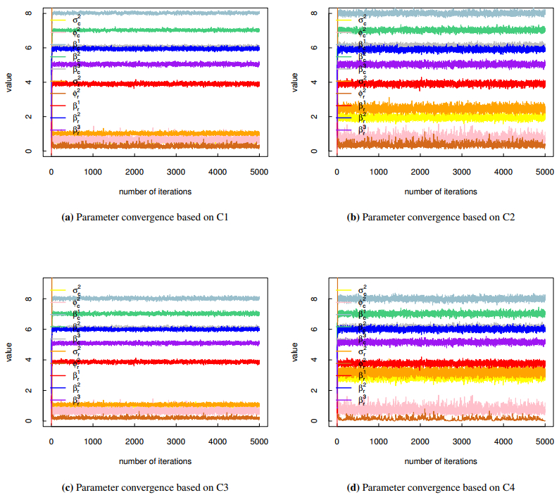
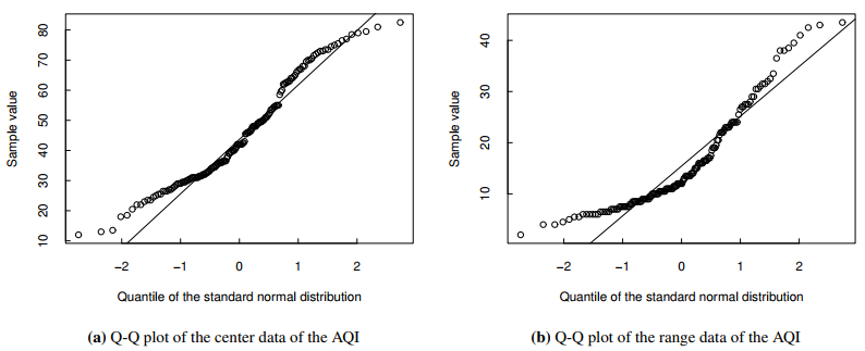
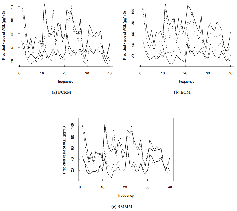
In the era of big data, interval-valued data is quite common in real life and can be used to describe the uncertainty of variables. In this paper, we introduced random effects panel interval-valued data models based on the center and range method and constructed a Bayesian method for the models, including estimation and prediction. Some simulation studies indicate that the proposed Bayesian method performs well. Finally, our proposed panel interval-valued data Bayesian models were applied in forecasting of the Air Quality Index, and the experimental evaluation of actual data sets shows the advantages and the performance of our proposed models.
Citation: Dengke Xu, Linlin Shen, Yuanyang Tangzhu, Shiqi Ke. Bayesian analysis of random effects panel interval-valued data models[J]. Electronic Research Archive, 2025, 33(5): 3210-3224. doi: 10.3934/era.2025141
In the era of big data, interval-valued data is quite common in real life and can be used to describe the uncertainty of variables. In this paper, we introduced random effects panel interval-valued data models based on the center and range method and constructed a Bayesian method for the models, including estimation and prediction. Some simulation studies indicate that the proposed Bayesian method performs well. Finally, our proposed panel interval-valued data Bayesian models were applied in forecasting of the Air Quality Index, and the experimental evaluation of actual data sets shows the advantages and the performance of our proposed models.

| [1] |
Y. Y. Sun, X. Y. Zhang, A. T. K. Wan, S. Y. Wang, Model averaging for interval-valued data, Eur. J. Oper. Res., 301 (2022), 772–784. https://doi.org/10.1016/j.ejor.2021.11.015 doi: 10.1016/j.ejor.2021.11.015

|
| [2] | L. Billard, E. Diday, Regression Analysis for Interval-Valued Data, Data Analysis, Classification and Related Methods, Berlin, Heidelberg: Springer, (2000), 369–374. https://doi.org/10.1007/978-3-642-59789-3-58 |
| [3] |
L. Billard, E. Diday, From the statistics of data to the statistics of knowledge: Symbolic data analysis, J. Am. Stat. Assoc., 98 (2003), 470–487. https://doi.org/10.1198/016214503000242 doi: 10.1198/016214503000242
|
| [4] |
L. Billard, E. Diday, Descriptive statistics for interval-valued observations in the presence of rules, Comput. Stat., 21 (2006), 187–210. https://doi.org/10.1007/s00180-006-0259-6 doi: 10.1007/s00180-006-0259-6
|
| [5] |
E. D. Lima, F. D. T. de Carvalho, Centre and range method for fitting a linear regression model to symbolic interval data, Comput. Stat. Data Anal., 52 (2008), 1500–1515. https://doi.org/10.1016/j.csda.2007.04.014 doi: 10.1016/j.csda.2007.04.014
|
| [6] |
E. D. Lima, F. D. T. de Carvalho, Constrained linear regression models for symbolic interval-valued variablesk, Comput. Stat. Data Anal., 54 (2010), 333–347. https://doi.org/10.1016/j.csda.2009.08.010 doi: 10.1016/j.csda.2009.08.010
|
| [7] |
P. Giordani, Lasso-constrained regression analysis for interval-valued data, Adv. Data Anal. Classif., 9 (2015), 5–19. https://doi.org/10.1007/s11634-014-0164-8 doi: 10.1007/s11634-014-0164-8
|
| [8] |
A. L. S. Maia, F. D. T. de Carvalho, Holt's exponential smoothing and neural network models for forecasting interval-valued time series, Int. J. Forecasting, 27 (2011), 740–759. https://doi.org/10.1016/j.ijforecast.2010.02.012 doi: 10.1016/j.ijforecast.2010.02.012
|
| [9] |
L. C. Souza, R. M. C. R. Souza, G. J. A. Amaral, T. M. Silva, A parametrized approach for linear-regression of interval data, Knowl.-Based Syst., 131 (2017), 149–159. https://doi.org/10.1016/j.knosys.2017.06.012 doi: 10.1016/j.knosys.2017.06.012
|
| [10] |
L. T. Kong, X. J. Song, X. M. Wang, Nonparametric regression for interval-valued data based on local linear smoothing approach, Neurocomputing, 501 (2022), 834–843. https://doi.org/10.1016/j.neucom.2022.06.073 doi: 10.1016/j.neucom.2022.06.073
|
| [11] |
L. T. Kong, X. W. Gao, A regularized MM estimate for interval-valued regression, Expert Syst. Appl., 238 (2024). https://doi.org/10.1016/j.eswa.2023.122044 doi: 10.1016/j.eswa.2023.122044
|
| [12] | E. Nuroglu, R. M. Kunst, The effects of exchange rate volatility on international trade flows: evidence from panel data analysis and fuzzy approach, in Proceedings of Rijeka Faculty of Economics: Journal of Economics and Business, 30 (2012), 9–31. |
| [13] |
F. He, D. D. Ma, X. N. Xu, Interval environmental efficiency across provinces in China under the constraint of haze with SBM-undesirable interval model, J. Arid Land Res. Environ., 30 (2016), 28–33. https://doi.org/10.13581/j.cnki.rdm.20160906.004 doi: 10.13581/j.cnki.rdm.20160906.004
|
| [14] |
S. N. Zhao, R. Q. Liu, Z. F. Shang, Statistical inference on panel data models: A kernel ridge regression method, J. Bus. Econ. Stat., 39 (2019), 325–337. https://doi.org/10.1080/07350015.2019.1660176 doi: 10.1080/07350015.2019.1660176
|
| [15] |
E. Aristodemou, Semiparametric identification in panel data discrete response models, J. Econom., 220 (2021), 253–271. https://doi.org/10.1016/j.jeconom.2020.04.002 doi: 10.1016/j.jeconom.2020.04.002
|
| [16] |
L. R. Liu, H. R. Moon, F. Schorfheide, Forecasting with a panel Tobit model, Quant. Econom., 14 (2023), 117–159. https://doi.org/10.3982/QE1505 doi: 10.3982/QE1505
|
| [17] |
B. H. Beyaztas, S. Bandyopadhyay, Robust estimation for linear panel data models, Stat. Med., 39 (2020), 4421–4438. https://doi.org/10.1002/sim.8732 doi: 10.1002/sim.8732
|
| [18] |
H. Liu, Y. Q. Pei, Q. F. Xu, Estimation for varying coefficient panel data model with cross-sectional dependence, Metrika, 83 (2020), 377–410. https://doi.org/10.1007/s00184-019-00739-0 doi: 10.1007/s00184-019-00739-0
|
| [19] |
S. Y. Ke, P. C. B. Phillips, L. J. Su, Robust inference of panel data models with interactive fixed effects under long memory: A frequency domain approach, J. Econom., 241 (2024). https://doi.org/10.1016/j.jeconom.2024.105761 doi: 10.1016/j.jeconom.2024.105761
|
| [20] |
A. B. Ji, J. J. Zhang, X. He, Y. H. Zhang, Fixed effects panel interval-valued data models and applications, Knowl.-Based Syst., 237 (2022). https://doi.org/10.1016/j.knosys.2021.107798 doi: 10.1016/j.knosys.2021.107798
|
| [21] |
T. Park, G. Casella. The bayesian lasso, J. Am. Stat. Assoc., 103 (2008), 681–686. https://doi.org/10.1198/016214508000000337 doi: 10.1198/016214508000000337
|
| [22] |
D. K. Xu, Z. Z. Zhang, A semiparametric Bayesian approach to joint mean and variance model, Stat. Probab. Lett., 83 (2013), 1624–1631. https://doi.org/10.1016/j.spl.2013.02.023 doi: 10.1016/j.spl.2013.02.023
|
| [23] |
I. Castillo, J. Schmidt-Hieber, A. V. der Vaart, Bayesian linear regression with sparse priors, Ann. Stat., 43 (2015), 1986–2018. https://doi.org/10.1214/15-AOS1334 doi: 10.1214/15-AOS1334
|
| [24] |
M. Pfarrhofer, P. Piribauer, Flexible shrinkage in high-dimensional Bayesian spatial autoregressive models, Spatial Stat., 29 (2019), 109–128. https://doi.org/10.1016/j.spasta.2018.10.004 doi: 10.1016/j.spasta.2018.10.004
|
| [25] |
Z. Q. Wang, N. S. Tang, Bayesian quantile regression with mixed discrete and Nonignorable missing covariates, Bayesian Anal., 15 (2020), 579–604. https://doi.org/10.1214/19-BA1165 doi: 10.1214/19-BA1165
|
| [26] |
D. Zhang, L. C. Wu, K. Y. Ye, M. Wang, Bayesian quantile semiparametric mixed-effects double regression models, Stat. Theory Relat. Fields, 5 (2021), 303–315. https://doi.org/10.1080/24754269.2021.1877961 doi: 10.1080/24754269.2021.1877961
|
| [27] |
L. Z. Tang, Y. J. Li, L. J. Zhao, Study on the Bayesian Elastic Net quantile regression for panel data: methods and applications, Stat. Res., 37 (2020), 94–113. https://doi.org/10.19343/j.cnki.11-1302/c.2020.03.008 doi: 10.19343/j.cnki.11-1302/c.2020.03.008
|
| [28] |
C. Q. Tao, Y. T. Xu, Study on Bayesian adaptive lasso quantile regression using asymmetric exponential power distribution for panel data, Stat. Res., 39 (2022), 128–144. https://doi.org/10.19343/j.cnki.11-1302/c.2022.09.010 doi: 10.19343/j.cnki.11-1302/c.2022.09.010
|
| [29] |
J. Zhang, M. Liu, M. Dong, Variational Bayesian inference for interval regression with an asymmetric Laplace distribution, Neurocomputing, 323 (2019), 214–230. https://doi.org/10.1016/j.neucom.2018.09.083 doi: 10.1016/j.neucom.2018.09.083
|
| [30] |
M. Xu, Z. F. Qin, A bivariate Bayesian method for interval-valued regression models, Knowl.-Based Syst., 235 (2022). https://doi.org/10.1016/j.knosys.2021.107396 doi: 10.1016/j.knosys.2021.107396
|
| [31] |
J. H. Ding, Z. Q. Zhang, Bayesian Statistical Models with Uncertainty Variables, J. Intell. Fuzzy Syst., 39 (2020), 1109–1117. https://doi.org/10.3233/JIFS-192014 doi: 10.3233/JIFS-192014
|
| [32] |
F. D. T. de Carvalho, R. M. C. R. de Souza, M. Chavent, Y. Lechevallier, Adaptive Hausdorff distances and dynamic clustering of symbolic interval data, Pattern Recognit. Lett., 27 (2006), 167–179. https://doi.org/10.1016/j.patrec.2005.08.014 doi: 10.1016/j.patrec.2005.08.014
|
| [33] |
C. Y. Hu, L. T. He, An application of interval methods to stock market forecasting, Reliab. Comput., 13 (2007), 423–434. https://doi.org/10.1007/s11155-007-9039-4 doi: 10.1007/s11155-007-9039-4
|
Figures(3) / Tables(10)
Dengke Xu, Linlin Shen, Yuanyang Tangzhu, Shiqi Ke. Bayesian analysis of random effects panel interval-valued data models[J]. Electronic Research Archive, 2025, 33(5): 3210-3224. doi: 10.3934/era.2025141


 DownLoad: