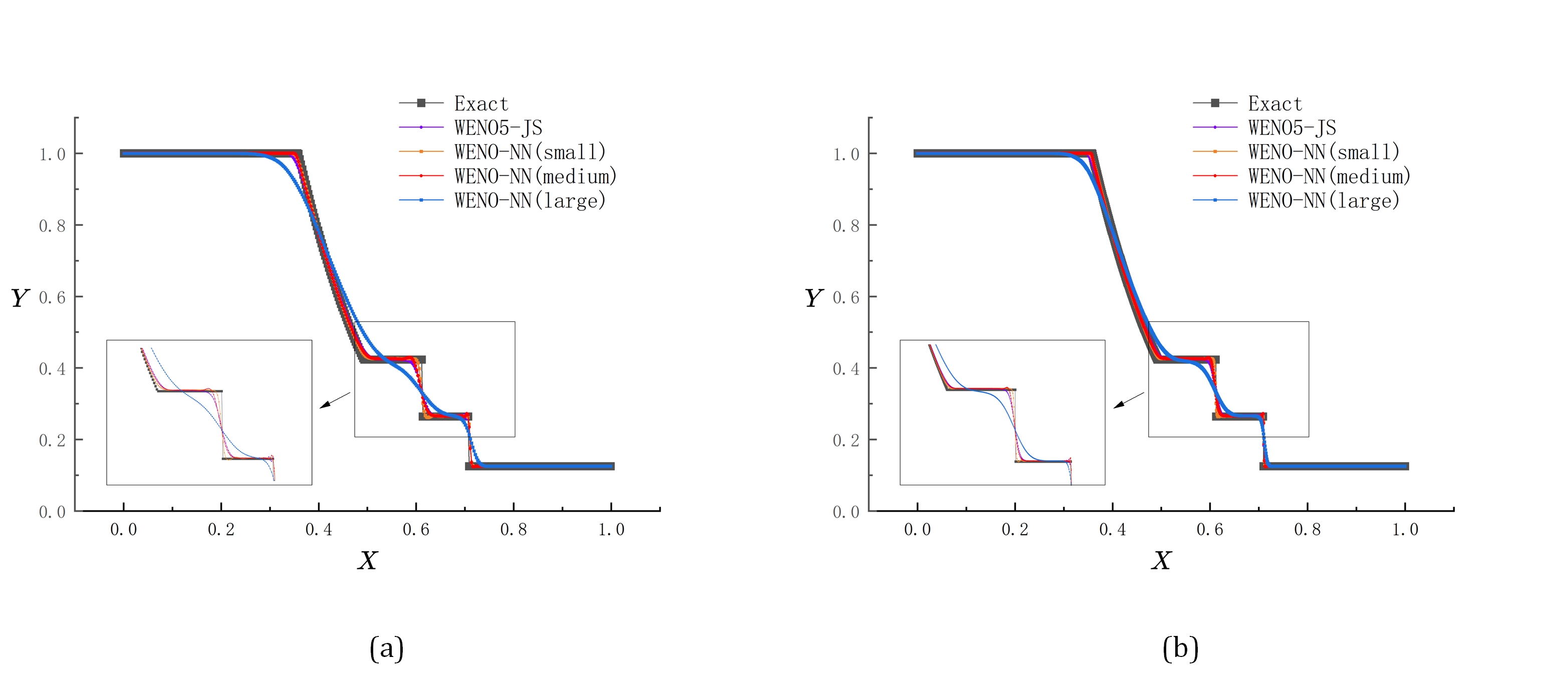
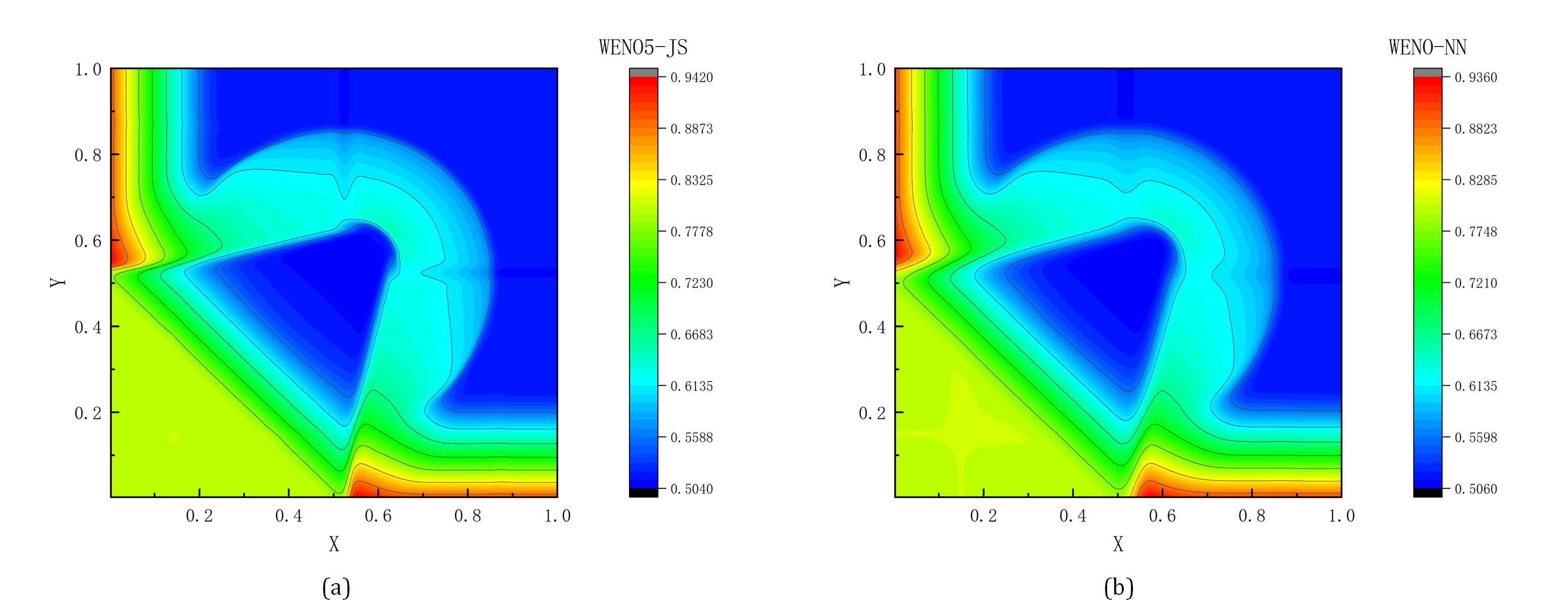
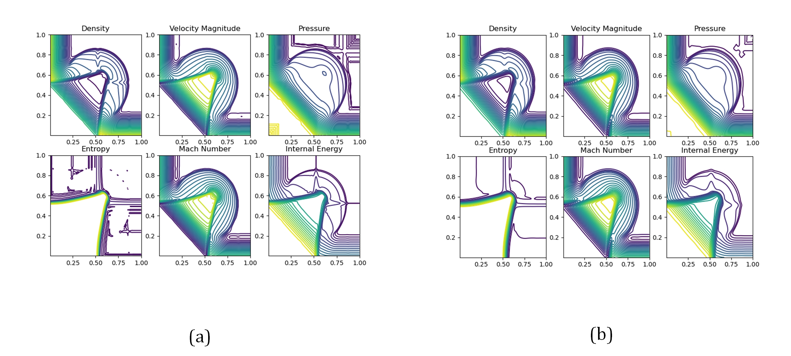
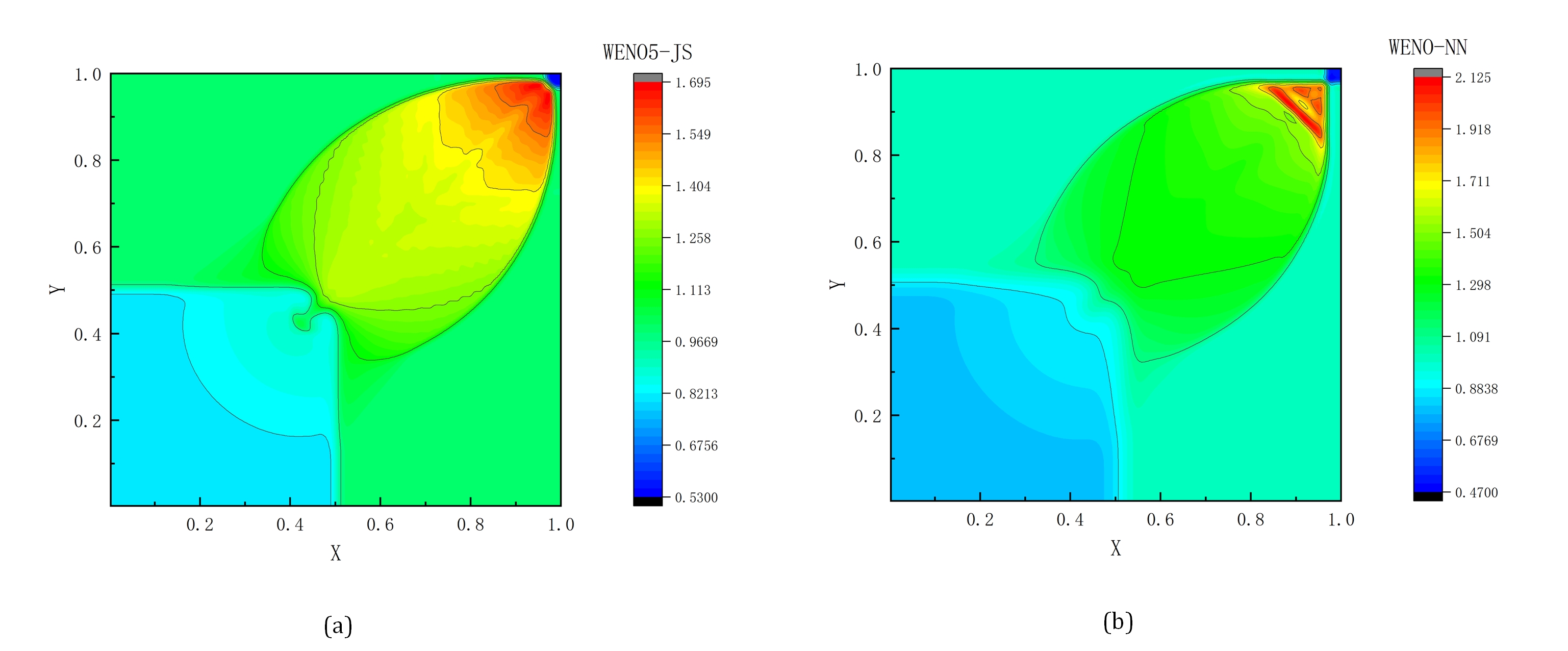
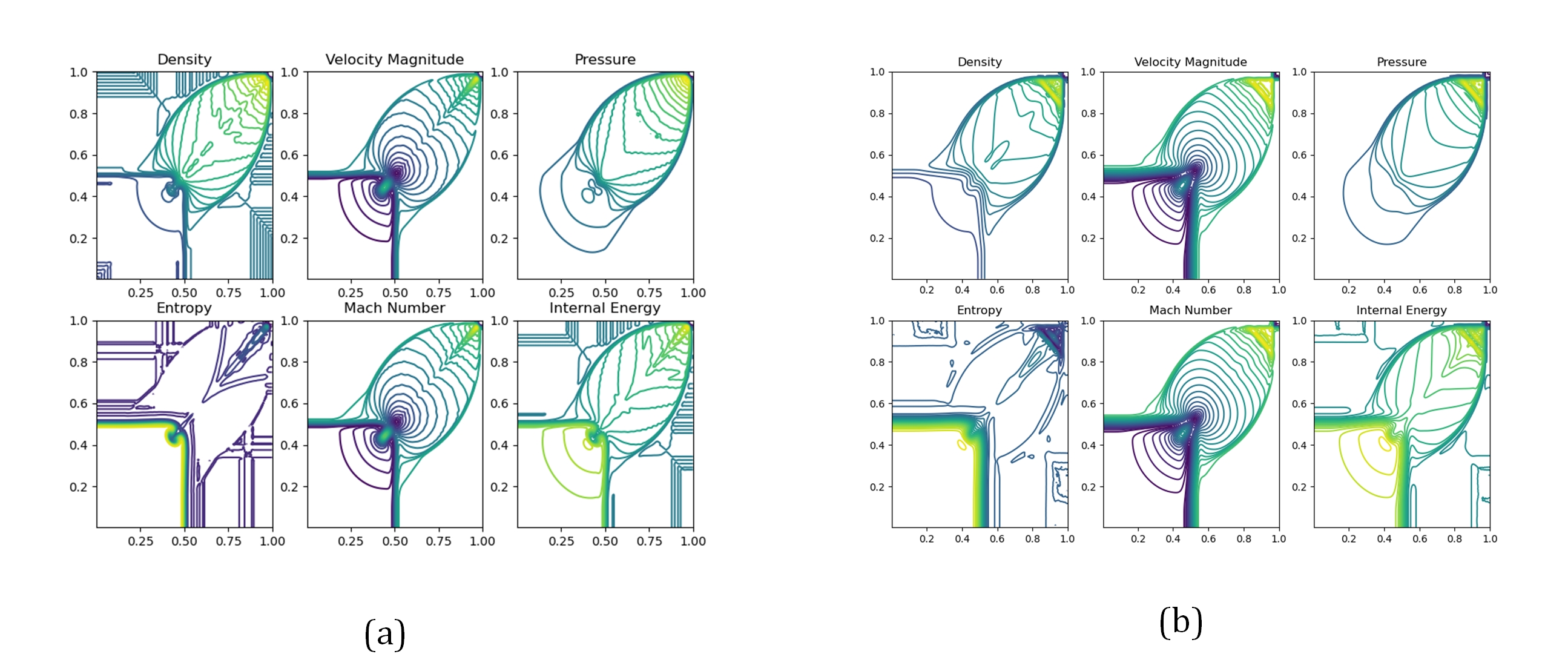
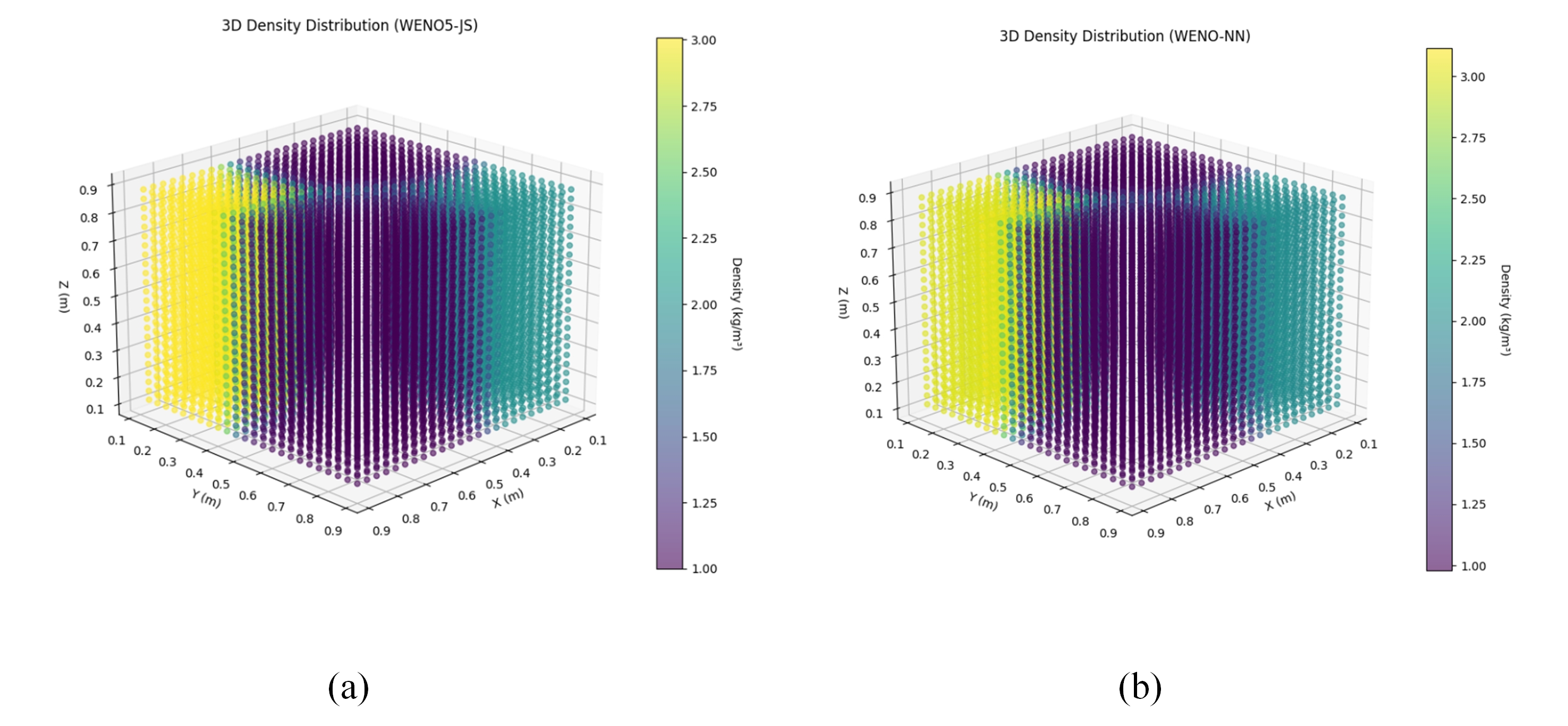
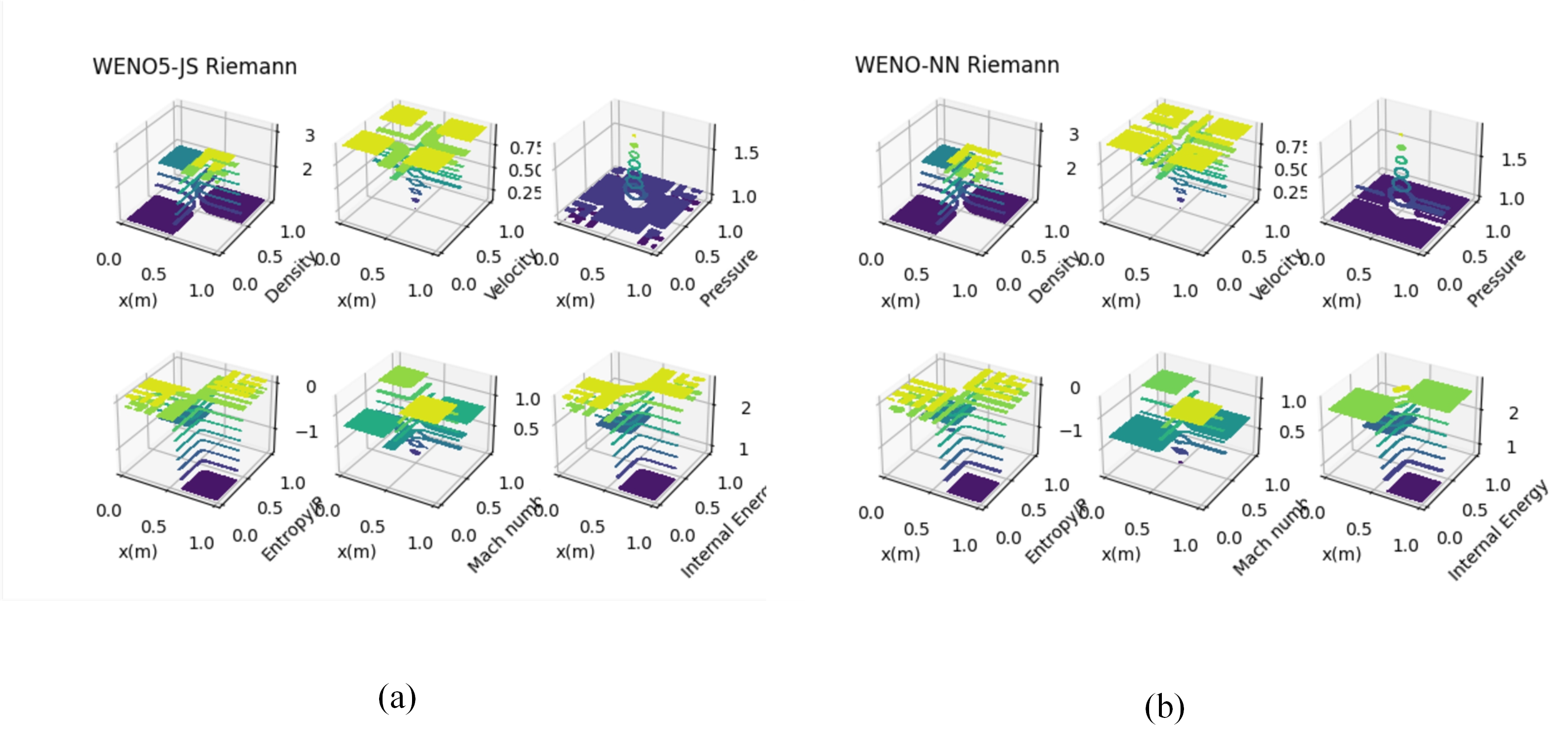
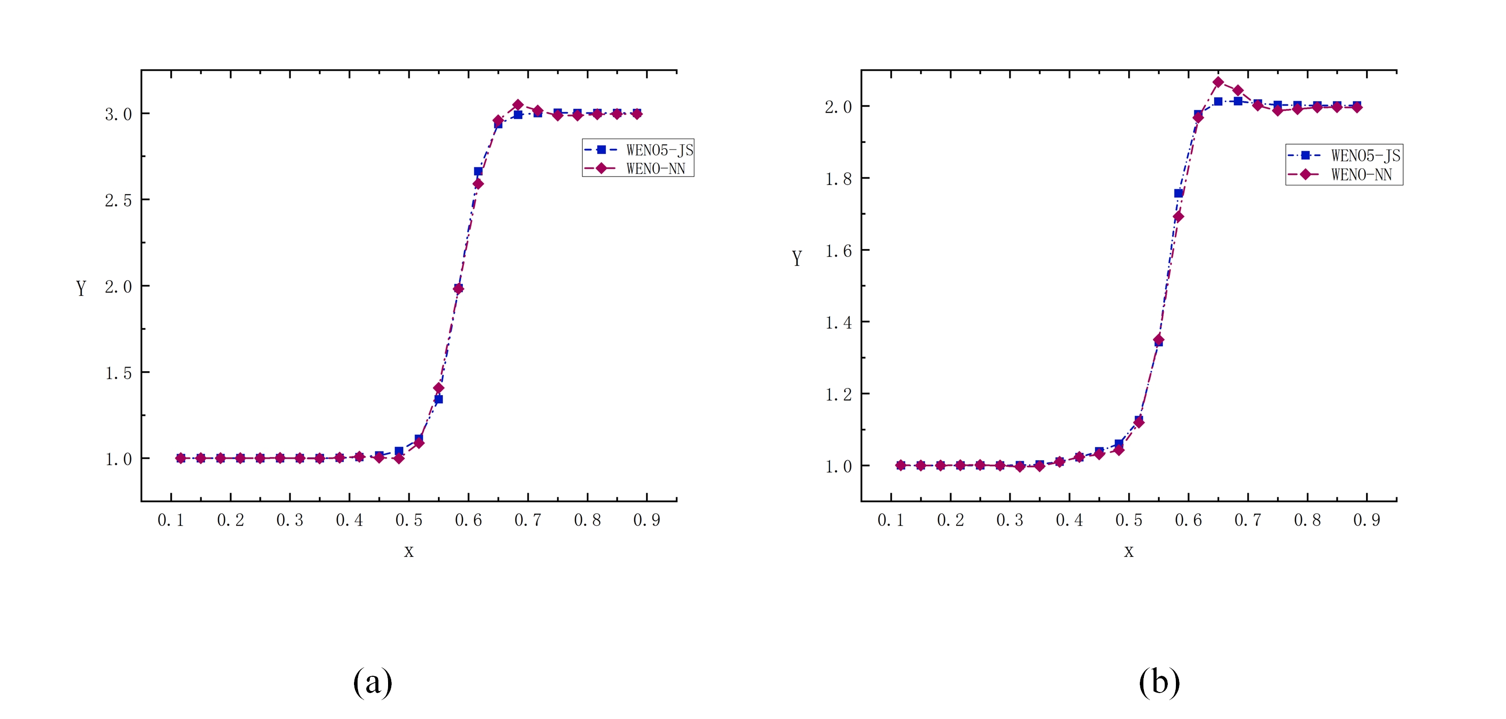
The weighted essentially non-oscillatory (WENO) scheme is widely used in fluid mechanics and other numerical simulation fields because of its high precision and low oscillation characteristics when dealing with hyperbolic conservation law equations containing discontinuities and high-gradient regions. However, the calculation of nonlinear weights in the WENO reconstruction process is complex and entails a high computational cost, especially when addressing two-dimensional and higher-dimensional problems, resulting in a limited overall computational efficiency. To improve computational efficiency, this study introduces a novel neural network-enhanced weighted essentially non-oscillatory method, abbreviated as WENO-NN. This method replaces the reconstruction process in the WENO scheme. Specifically, we used a subset of the data generated by the WENO method to train a neural network that approximates the functionality of WENO. This approach significantly improved the computational efficiency while preserving accuracy. Further, we evaluated the performance of the WENO-NN scheme on both one-dimensional, two-dimensional, and three-dimensional test cases, including scenarios involving the interaction of strong shocks and shock-density waves. The results demonstrated that the WENO-NN scheme exhibits good versatility across all benchmark tests and resolutions. Its accuracy is comparable to that of the classic WENO scheme, while its computational efficiency is improved by 3 times.
Citation: Shanpu Gao, Yubo Li, Anping Wu, Hao Jiang, Feng Liu, Xinlong Feng. An intelligent optimization method for accelerating physical quantity reconstruction in computational fluid dynamics[J]. Electronic Research Archive, 2025, 33(5): 2881-2924. doi: 10.3934/era.2025127
The weighted essentially non-oscillatory (WENO) scheme is widely used in fluid mechanics and other numerical simulation fields because of its high precision and low oscillation characteristics when dealing with hyperbolic conservation law equations containing discontinuities and high-gradient regions. However, the calculation of nonlinear weights in the WENO reconstruction process is complex and entails a high computational cost, especially when addressing two-dimensional and higher-dimensional problems, resulting in a limited overall computational efficiency. To improve computational efficiency, this study introduces a novel neural network-enhanced weighted essentially non-oscillatory method, abbreviated as WENO-NN. This method replaces the reconstruction process in the WENO scheme. Specifically, we used a subset of the data generated by the WENO method to train a neural network that approximates the functionality of WENO. This approach significantly improved the computational efficiency while preserving accuracy. Further, we evaluated the performance of the WENO-NN scheme on both one-dimensional, two-dimensional, and three-dimensional test cases, including scenarios involving the interaction of strong shocks and shock-density waves. The results demonstrated that the WENO-NN scheme exhibits good versatility across all benchmark tests and resolutions. Its accuracy is comparable to that of the classic WENO scheme, while its computational efficiency is improved by 3 times.

| [1] |
X. Feng, X. Lu, Y. He, Difference finite element method for the 3D steady Navier-Stokes equations, SIAM J. Numer. Anal., 61 (2023), 167–193. https://doi.org/10.1137/21m1450872 doi: 10.1137/21m1450872

|
| [2] |
N. Li, J. Wu, X. Feng, Filtered time-stepping method for incompressible Navier-Stokes equations with variable density, J. Comput. Phys., 473 (2023), 111764. https://doi.org/10.1016/j.jcp.2022.111764 doi: 10.1016/j.jcp.2022.111764
|
| [3] |
G. Peng, Z. Gao, W. Yan, X. Feng, A positivity-preserving finite volume scheme for three-temperature radiation diffusion equations, Appl. Numer. Math., 152 (2020), 125–140, https://doi.org/10.1016/j.apnum.2020.01.013 doi: 10.1016/j.apnum.2020.01.013
|
| [4] |
A. Harten, High resolution schemes for hyperbolic conservation laws, J. Comput. Phys., 49 (1983), 357–393, https://doi.org/10.1016/0021-9991(83)90136-5 doi: 10.1016/0021-9991(83)90136-5
|
| [5] |
A. Harten, B. Engquist, S. Osher, S. R. Chakravarthy, Uniformly high order accurate essentially non-oscillatory schemes, Ⅲ, J. Comput. Phys., 131 (1997), 3–47. https://doi.org/10.1006/jcph.1996.5632 doi: 10.1006/jcph.1996.5632
|
| [6] |
G. S. Jiang, C. W. Shu, Efficient implementation of weighted ENO schemes, J. Comput. Phys., 126 (1996), 202–228. https://doi.org/10.1006/jcph.1996.0130 doi: 10.1006/jcph.1996.0130
|
| [7] |
Y. Ha, C. H. Kim, Y. J. Lee, J. Yoon, An improved weighted essentially non-oscillatory scheme with a new smoothness indicator, J. Comput. Phys., 232 (2013), 68–86. https://doi.org/10.1016/j.jcp.2012.06.016 doi: 10.1016/j.jcp.2012.06.016
|
| [8] |
C. H. Kim, Y. Ha, J. Yoon, Modified non-linear weights for fifth-order weighted essentially non-oscillatory schemes, J. Sci. Comput., 67 (2016), 299–323. https://doi.org/10.1007/s10915-015-0079-3 doi: 10.1007/s10915-015-0079-3
|
| [9] |
S. Rathan, G. N. Raju, A modified fifth-order WENO scheme for hyperbolic conservation laws, Comput. Math. Appl., 75 (2018), 1531–1549. https://doi.org/10.1016/j.camwa.2017.11.020 doi: 10.1016/j.camwa.2017.11.020
|
| [10] |
R. Borges, M. Carmona, B. Costa, W. S. Don, An improved weighted essentially non-oscillatory scheme for hyperbolic conservation laws, J. Comput. Phys., 227 (2008), 3191–3211. https://doi.org/10.1016/j.jcp.2007.11.038 doi: 10.1016/j.jcp.2007.11.038
|
| [11] |
M. Castro, B. Costa, W. S. Don, High order weighted essentially non-oscillatory WENO-Z schemes for hyperbolic conservation laws, J. Comput. Phys., 230 (2011), 1766–1792. https://doi.org/10.1016/j.jcp.2010.11.028 doi: 10.1016/j.jcp.2010.11.028
|
| [12] |
S. Rathan, G. N. Raju, Improved weighted ENO scheme based on parameters involved in nonlinear weights, Appl. Math. Comput., 331 (2018), 120–129. https://doi.org/10.1016/j.amc.2018.03.034 doi: 10.1016/j.amc.2018.03.034
|
| [13] |
G. Li, J. Qiu, Hybrid weighted essentially non-oscillatory schemes with different indicators, J. Comput. Phys., 229 (2010), 8105–8129. https://doi.org/10.1016/j.jcp.2010.07.012 doi: 10.1016/j.jcp.2010.07.012
|
| [14] |
A. A. I. Peer, M. Z. Dauhoo, M. Bhuruth, A method for improving the performance of the WENO5 scheme near discontinuities, Appl. Math. Lett., 22 (2009), 1730–1733. https://doi.org/10.1016/j.aml.2009.05.016 doi: 10.1016/j.aml.2009.05.016
|
| [15] |
J. Kim, D. Lee, Optimized compact finite difference schemes with maximum resolution, AIAA J., 34 (1996), 887–893. https://doi.org/10.2514/3.13164 doi: 10.2514/3.13164
|
| [16] |
Y. Liu, Globally optimal finite-difference schemes based on least squares, Geophysics, 78 (2013), T113–T132. https://doi.org/10.1190/geo2012-0480.1 doi: 10.1190/geo2012-0480.1
|
| [17] |
C. K. W. Tam, J. C. Webb, Dispersion-relation-preserving finite difference schemes for computational acoustics, J. Comput. Phys., 107 (1993), 262–281. https://doi.org/10.1006/jcph.1993.1142 doi: 10.1006/jcph.1993.1142
|
| [18] |
J. H. Zhang, Z. X. Yao, Optimized explicit finite-difference schemes for spatial derivatives using maximum norm, J. Comput. Phys., 250 (2013), 511–526. https://doi.org/10.1016/j.jcp.2013.04.029 doi: 10.1016/j.jcp.2013.04.029
|
| [19] |
J. Fang, Z. Li, L. Lu, An optimized low-dissipation monotonicity-preserving scheme for numerical simulations of high-speed turbulent flows, J. Sci. Comput., 56 (2013), 67–95. https://doi.org/10.1007/s10915-012-9663-y doi: 10.1007/s10915-012-9663-y
|
| [20] |
Z. J. Wang, R. F. Chen, Optimized weighted essentially nonoscillatory schemes for linear waves with discontinuity, J. Comput. Phys., 174 (2001), 381–404. https://doi.org/10.1006/jcph.2001.6918 doi: 10.1006/jcph.2001.6918
|
| [21] |
T. Kossaczká, M. Ehrhardt, M. Günther, Enhanced fifth order WENO shock-capturing schemes with deep learning, Results Appl. Math., 12 (2021), 100201. https://doi.org/10.1016/j.rinam.2021.100201 doi: 10.1016/j.rinam.2021.100201
|
| [22] |
S. Li, X. Feng, Dynamic weight strategy of physics-informed neural networks for the 2d navier-stokes equations, Entropy, 24 (2022), 1254. https://doi.org/10.3390/e24091254 doi: 10.3390/e24091254
|
| [23] |
S. Tang, X. Feng, W. Wu, H. Xu, Physics-informed neural networks combined with polynomial interpolation to solve nonlinear partial differential equations, Comput. Math. Appl., 132 (2023), 48–62. https://doi.org/10.1016/j.camwa.2022.12.008 doi: 10.1016/j.camwa.2022.12.008
|
| [24] |
J. Zhao, W. Wu, X. Feng, H. Xu, Solving Euler equations with gradient-weighted multi-input high-dimensional feature neural network, Phys. Fluids, 36 (2024), 035150. https://doi.org/10.1063/5.0194523 doi: 10.1063/5.0194523
|
| [25] |
Y. Wang, C. Xu, M. Yang, J. Zhang, Less emphasis on hard regions: Curriculum learning of PINNs for singularly perturbed convection-diffusion-reaction problems, East Asian J. Appl. Math., 14 (2024), 104–123. https://doi.org/10.4208/eajam.2023-062.170523 doi: 10.4208/eajam.2023-062.170523
|
| [26] |
T. Zhang, H. Xu, Y. Zhang, X. Feng, Residual-based reduced order models for parameterized Navier-Stokes equations with nonhomogeneous boundary condition, Phys. Fluids, 36 (2024), 093624. https://doi.org/10.1063/5.0225839 doi: 10.1063/5.0225839
|
| [27] |
D. A. Bezgin, S. J. Schmidt, N. A. Adams, WENO3-NN: A maximum-order three-point data-driven weighted essentially non-oscillatory scheme, J. Comput. Phys., 452 (2022), 110920. https://doi.org/10.1016/j.jcp.2021.110920 doi: 10.1016/j.jcp.2021.110920
|
| [28] |
Q. Liu, The WENO reconstruction based on the artificial neural network, Adv. Appl. Math., 9 (2020), 574–583. https://doi.org/10.12677/aam.2020.94069 doi: 10.12677/aam.2020.94069
|
| [29] |
X. Nogueira, J. Fernández-Fidalgo, L. Ramos, I. Couceiro, L. Ramírez, Machine learning-based WENO5 scheme, Comput. Math. Appl., 168 (2024), 84–99. https://doi.org/10.1016/j.camwa.2024.05.031 doi: 10.1016/j.camwa.2024.05.031
|
| [30] |
B. Stevens, T. Colonius, Enhancement of shock-capturing methods via machine learning, Theor. Comput. Fluid Dyn., 34 (2020), 483–496. https://doi.org/10.1007/s00162-020-00531-1 doi: 10.1007/s00162-020-00531-1
|
| [31] |
S. Takagi, L. Fu, H. Wakimura, F. Xiao, A novel high-order low-dissipation TENO-THINC scheme for hyperbolic conservation laws, J. Comput. Phys., 452 (2022), 110899. https://doi.org/10.1016/j.jcp.2021.110899 doi: 10.1016/j.jcp.2021.110899
|
| [32] |
C. W. Shu, S. Osher, Efficient implementation of essentially non-oscillatory shock-capturing schemes, J. Comput. Phys., 77 (1988), 439–471. https://doi.org/10.1016/0021-9991(88)90177-5 doi: 10.1016/0021-9991(88)90177-5
|
| [33] |
X. D. Liu, S. Osher, T. Chan, Weighted essentially non-oscillatory schemes, J. Comput. Phys., 115 (1994), 200–212. https://doi.org/10.1006/jcph.1994.1187 doi: 10.1006/jcph.1994.1187
|
| [34] |
X. Zhong, High-order finite-difference schemes for numerical simulation of hypersonic boundary-layer transition, J. Comput. Phys., 144 (1998), 662–709. https://doi.org/10.1006/jcph.1998.6010 doi: 10.1006/jcph.1998.6010
|
| [35] |
S. Gottlieb, C. W. Shu, E. Tadmor, Strong stability-preserving high-order time discretization methods, SIAM Rev., 43 (2001), 89–112. https://doi.org/10.1137/s003614450036757x doi: 10.1137/s003614450036757x
|
| [36] |
G. A. Sod, A survey of several finite difference methods for systems of nonlinear hyperbolic conservation laws, J. Comput. Phys., 27 (1978), 1–31. https://doi.org/10.1016/0021-9991(78)90023-2 doi: 10.1016/0021-9991(78)90023-2
|
| [37] |
P. Lax, Weak solutions of nonlinear hyperbolic equations and their numerical computation, Commun. Pure Appl. Math., 7 (1954), 159–193. https://doi.org/10.1002/cpa.3160070112 doi: 10.1002/cpa.3160070112
|
| [38] |
A. Kurganov, E. Tadmor, Solution of two-dimensional Riemann problems for gas dynamics without Riemann problem solvers, Numer. Methods Partial Differ. Equations, 18 (2002), 584–608. https://doi.org/10.1002/num.10025 doi: 10.1002/num.10025
|
| [39] |
G. Capdeville, A central WENO scheme for solving hyperbolic conservation laws on non-uniform meshes, J. Comput. Phys., 227 (2008), 2977–3014. https://doi.org/10.1016/j.jcp.2007.11.029 doi: 10.1016/j.jcp.2007.11.029
|
| [40] |
P. D. Lax, X. D. Liu, Solution of two-dimensional Riemann problems of gas dynamics by positive schemes, SIAM J. Sci. Comput., 19 (1998), 319–340. https://doi.org/10.1137/s1064827595291819 doi: 10.1137/s1064827595291819
|
| [41] |
Q. Zhang, P. Huang, Y. He, A difference mixed finite element method for the three dimensional poisson equation, East Asian J. Appl. Math., 15 (2025), 268–289. https://doi.org/10.4208/eajam.2023-247.050224 doi: 10.4208/eajam.2023-247.050224
|
| [42] |
M. Jiang, J. Wu, N. Li, X. Feng, An analysis of second-order sav-filtered time-stepping finite element method for unsteady natural convection problems, Commun. Nonlinear Sci. Numer. Simul., 140 (2025), 108365. https://doi.org/10.1016/j.cnsns.2024.108365 doi: 10.1016/j.cnsns.2024.108365
|
| [43] |
Y. Liu, Y. He, X. Feng, Difference finite element methods based on different discretization elements for the four-dimensional poisson equation, East Asian J. Appl. Math., 15 (2025), 415–438. https://doi.org/10.4208/eajam.2023-233.200224 doi: 10.4208/eajam.2023-233.200224
|
| [44] |
F. Tang, F. Liu, A. Wu, Q. Wang, J. Huang, Y. Li, Super-resolution reconstruction of flow fields coupled with feature recognition, Phys. Fluids, 36 (2024), 077148. https://doi.org/10.1063/5.0219162 doi: 10.1063/5.0219162
|
| [45] |
L. Tang, F. Liu, A. Wu, Y. Li, W. Jiang, Q. Wang, et al., A combined modeling method for complex multi-fidelity data fusion, Mach. Learn.: Sci. Technol., 5 (2024), 035071. https://doi.org/10.1088/2632-2153/ad718f doi: 10.1088/2632-2153/ad718f
|
Figures(23) / Tables(27)
Shanpu Gao, Yubo Li, Anping Wu, Hao Jiang, Feng Liu, Xinlong Feng. An intelligent optimization method for accelerating physical quantity reconstruction in computational fluid dynamics[J]. Electronic Research Archive, 2025, 33(5): 2881-2924. doi: 10.3934/era.2025127


 DownLoad: