Analysis of a reaction-diffusion AIDS model with media coverage and population heterogeneity

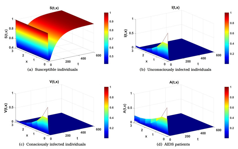
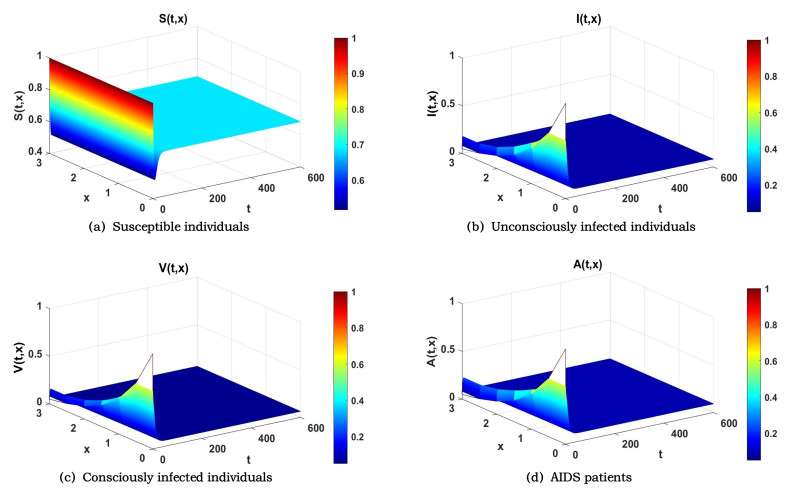
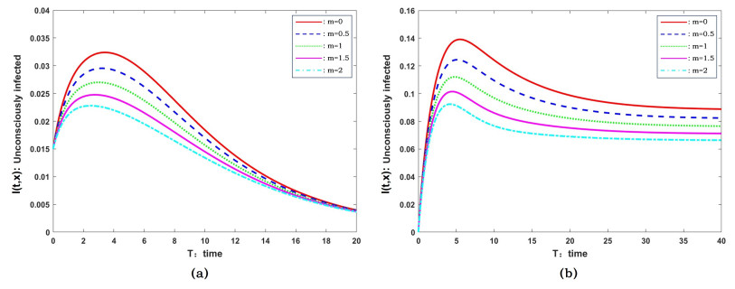
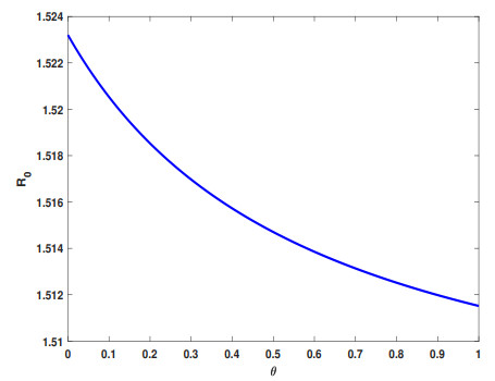
1.   Introduction

AIDS, also known as acquired immunodeficiency syndrome, is a severe immune system disease caused by the human immunodeficiency virus (HIV)^[1]. The virus invades the human body and destroys the immune system. This causes the infected person to gradually lose the ability to fight against various diseases, ultimately leading to death^[2]. The main routes of HIV/AIDS transmission include blood, sexual contact, and mother-to-child transmission^[3]. In the initial weeks following infection, individuals may remain asymptomatic. They might spread the virus to others easily at this stage since they regard themselves as healthy individuals. As the infection advances, the immune system deteriorates and individuals may experience symptoms such as fever, cough, diarrhea, weight loss and swollen lymph nodes. AIDS is the final stage of HIV infection^[4]. Particularly, while significant efforts have been made to control it, AIDS remains incurable today. According to the World Health Organization (WHO)^[5], by the end of 2023, there will be about 39.9 million people living with HIV worldwide. The data indicates that AIDS will be a serious public health issue if left untreated and uncontrolled.

Mathematical modeling is an effective method for quantitative and qualitative analysis of disease transmission mechanisms, which is essential for controlling diseases in the field of epidemiology. It is worth noting that mathematicians have paid much attention to the spread of HIV/AIDS infection. From 1986 to 1988, Anderson and May^[6,7,8] successively proposed deterministic mathematical models to describe HIV/AIDS transmission. In recent years, with the complex changes in the social environment, an increasing number of factors can affect HIV/AIDS transmission. Therefore, many scholars have incorporated various factors and established models to study the influence of these factors on the spread of HIV/AIDS, such as a stochastic AIDS model with bilinear incidence and self-protection awareness^[9], an AIDS model with Age-Structured^[10], a spatial diffusion HIV/AIDS model with antiretroviral therapy and pre-exposure prophylaxis treatments^[11], a stochastic Sex-structured AIDS epidemic model^[12], an AIDS model with systematic perturbations and multiple susceptible population^[13], and others. In particular, the severity of the spread of AIDS varies from region to region due to differences in economic development, population education, and openness^[14]. Thus, spatial diffusion is a crucial factor in studying the spread of AIDS/HIV. Wu et al.^[15] proposed a spatial diffusion HIV model with periodic delays and the three-stage infection process to examine the impacts of periodic antiviral treatment and spatial heterogeneity on HIV infection. In ^[16], Chen et al. investigated a dynamic model of HIV transmission in the human body that included a spatially heterogeneous diffusion term and derived conditions for virus persistence in heterogeneous spaces. Authors in^[17] investigated a reaction-diffusion HIV infection model with (cytotoxic T lymphocytes) CTLs chemotactic movement and discussed the global well-posedness and global dynamical properties of the model. ^[18] studied an HIV/AIDS reaction-diffusion epidemic model, suggesting that the optimal controller aims to minimize the sizes of susceptible and infected populations.

It is known that AIDS is incurable. Currently, there are two approaches to controlling AIDS: one is pharmacological, such as continuous antiretroviral treatment (ART), and the other is non-pharmacological interventions, such as media coverage, awareness-control education, and others. In recent years, many scholars have increasingly incorporated media coverage into infectious disease modeling. Liu et al.^[19] studied an (susceptible-vaccinated-exposed-infected-recovered-infected) SVEIR-I infectious disease model with media coverage, revealing that media coverage can control the spread of diseases by reducing the effective contact rate through widespread dissemination of information. In Cui et al.^[20], an (susceptible-exposed-infected) SEI model is proposed and describes the impact of the media coverage coefficient $m$ on the spread and control of (severe acute respiratory syndrome) SARS through the effective exposure rate $\beta(I) = \mu e^{-mI}$. In ^[21], the authors added a media coverage level compartment $M$ to the $SEIR$ model, and the function $e^{-\mu M}$ was used to represent the effect of media coverage in the incidence rate. Sahu and Dhar^[22] introduced the media-induced transmission rate of the form $\beta e^{-m_1 \frac{I}{N} -m_2 \frac{H}{N}}$ into (susceptible-exposed-quarantined-infected-hospitalized-recovered-susceptible) SEQIHRS epidemic model, where $m_1$ and $m_2$ are coefficients representing media coverage effects of non-pharmaceutical interventions on infectious ($I$) and isolated ($H$) individuals, respectively. As mentioned in ^[23], mass media (e.g., newspapers and television) are essential for disseminating information about HIV/AIDS to the public. In particular, Wang et al.^[24] constructed a hybrid HIV/AIDS model with media coverage, age-structure, and self-protection mechanisms, concluding that media coverage can motivate individuals to take precautions against HIV infection and help control the spread of AIDS. Thus, incorporating the impact of media coverage into HIV/AIDS transmission modeling is increasingly important.

The researchers have significantly advanced the field of HIV/AIDS transmission modeling. However, a dynamical model of the spread of AIDS in the population that takes into account both spatial reaction-diffusion and the media coverage factor is not currently available. In addition, the establishment of HIV voluntary counseling and testing (VCT) clinics can lead to the development of behavioral control among individuals who are aware of their HIV infection, thereby reducing their ability to transmit. Therefore, we can study the impact on AIDS transmission by dividing the population into different awareness categories. Based on the discussions mentioned above, this paper considers the dynamics of AIDS transmission across different populations and the number of AIDS cases regularly reported in the media, we propose the following reaction-diffusion model of AIDS transmission with nonlinear incidence rates and the media coverage factor:

satisfy

and

where $\frac{\partial}{\partial v}$ represents the outward normal derivative on $\partial\Omega$. Based on the characteristics of AIDS transmission and the above facts, we classify the population into susceptible individuals, unconsciously infected individuals, consciously infected individuals, and AIDS patients, denoted by $S(t, x)$, $I(t, x)$, $V(t, x)$, $A(t, x)$, respectively. The total population of the region is $N(t, x) = S(t, x)+I(t, x)+V(t, x)+A(t, x)$.

It is supposed that HIV-infected individuals and AIDS patients are differentially infectious to susceptible individuals. Therefore, we use $\beta_{1}$, $\beta_{2}$, and $\beta_{3}$ to measure the effective disease transmission ability of unconsciously infected individuals, consciously infected individuals, and AIDS patients to susceptible individuals, respectively. In addition, in order to better characterize the weakening effect of media coverage on the disease transmission ability, we used transmission rate functions with an exponential form proposed by ^[20], namely, $\beta_{1}e^{-mA}$, $\beta_{2}e^{-mA}$, and $\beta_{3}e^{-mA}$. If $m = 0$, it represents not factoring in media coverage; if $m > 0$, it reflects the effects of having media coverage. As $m$ increases, that represents media coverage intensifies, and it further weakens the disease transmission ability. Also, media coverage primarily focuses on reporting the number of AIDS cases. With the rise in reported AIDS cases, public awareness and concern are heightened, leading to greater awareness of protective measures. This heightened awareness ultimately contributes to a reduction in the disease's transmission rate. Other parameters used in the model (1.1) are defined in Table 1. In addition, nonlinear incidence functions in the model (1.1) meet the following assumption.

where $\mathbf{T}(\cdot) = k(\cdot), n(\cdot), r(\cdot)$, and $x = I, V, A$.

2.   Positivity and boundedness of solutions

We denote $\mathbb{L}: = C(\bar{\Omega}, \mathbb{R}^{m})$ as the Banach space, and let its positive cone be $\mathbb{L^+}: = C(\bar{\Omega}, \mathbb{R}^{m}_+)$. Then, we denote $\mathbb{L}: = C(\bar{\Omega}, \mathbb{R}^{4})$ and $\mathbb{L^+}: = C(\bar{\Omega}, \mathbb{R}^{4}_+)$. Suppose that $\mathbb{M}_i(x):C(\bar{\Omega}, \mathbb{R}^{4}) \rightarrow C(\bar{\Omega}, \mathbb{R}^{4}_+)$ ($i$ = 1, 2, 3, 4) are the $C_{0}$ semigroups associated with $\mathcal{D}_1 \Delta-\mu$, $\mathcal{D}_2 \Delta-\theta-\delta-\mu$, $\mathcal{D}_3 \Delta-(1-a)\delta-\mu$, and $\mathcal{D}_4 \Delta-d-\mu$, respectively. From (1.1), we have

for any $\phi\in C(\bar{\Omega}, \mathbb{R})$ and $t > 0$, where $\Upsilon_i$ are the Green functions associated with $\mathcal{D}_i \Delta$ ($i$ = 1, 2, 3, 4) depending on (1.1). It follows from ^[25] that $\mathbb{M}_i(t)$ ($i$ = 1, 2, 3, 4) are strongly positive and compact.

We define $\mathcal{T} = (\mathcal{T}_1, \mathcal{T}_2, \mathcal{T}_3, \mathcal{T}_4)$ as follows:

with initial value $\phi_i \in \mathbb{L^+}$ and $\mathcal{T}_i:\mathbb{L^+}\rightarrow \mathbb{L}$ ($i$ = 1, 2, 3, 4).

Hence, we let $\mathbb{U}(t, x) = (S(t, x), I(t, x), V(t, x), A(t, x))$, $\mathbb{M}(t) = (\mathbb{M}_1(t), \mathbb{M}_2(t), \mathbb{M}_3(t), \mathbb{M}_4(t))$ and write the system (1.1) as

To obtain the existence and ultimate boundedness of the solutions for the system $(1.1)$, we give the following results.

Theorem 1. Given any $\phi\in\mathbb{L^+}$, the system $(1.1)$ has a unique mild solution $\mathbb{U}(t, \cdot, \phi) = (S(t, \cdot, \phi), I(t, \cdot, \phi), V(t, \cdot, \phi), A(t, \cdot, \phi))$; and

is point dissipative, where $\omega(t):\mathbb{L^+}\rightarrow \mathbb{L^+}$.

Proof. For any $H \geq 0$ and $\phi\in\mathbb{L^+}$, we have

Based on Corollary 4 of Martin and Smith^[25], we can see that $\mathbb{U}(t, \cdot, \phi)$ is a unique mild solution of (1.1) for $t\in\left [ 0, \tau_\phi \right)$ with initial value $\mathbb{U}(0, \cdot, \phi) = (\phi_1, \phi_2, \phi_3, \phi_4) \in\mathbb{L^+}$, where $\tau_\phi\leq+ \infty$.

Consider all equations of the system (1.1), and denote $N(t) = \int_{\Omega}[S(t, x)+I(t, x)+V(t, x)+A(t, x)]dx$, then

where $\left | \Omega \right |$ represents the measure of the region $\Omega$. Using the Gronwall inequality, the following result is obtained.

Similar to the proof of Lemma 2.1 in ^[26], and using mathematical induction, it can be shown that there exists a constant $\mathcal{M} > 0$ independent of the initial values, such that

This indicates that $S(t, x), I(t, x), V(t, x), A(t, x)$ are all uniformly bounded. Thus, we know that $\omega(t)\phi$ is point dissipative. □

3.   Basic reproduction number

There always exists a (disease-free equilibrium)DFE $E^0 = (S_0, 0, 0, 0)$ for the system (1.1), where $S_0 = \frac{\Lambda}{\mu}$. By the method of ^[27], the system (1.1) can be rewritten as

where $\mathbb{Y} = (I, V, A, S)^\top$. The new infection matrix $\mathcal{F}(x, \mathbb{Y})$ and the transition matrix $\mathcal{J}(x, \mathbb{Y})$ are as follows:

and

Next, we obtain the linearized matrices evaluated at $E^0 = (S_0, 0, 0, 0)$.

and

where $l$ represents the wave number. $F$ is a nonnegative matrix, and $J$ is a cooperative matrix. Thus, $FJ^{-1}$ is nonnegative. According to the concept of next-generation operators from ^[27,28,29], the basic reproduction number can be given by $\rho({FJ^{-1}})$, which represents the spectral radius of matrix $FJ^{-1}$. By simple computation, one has

We divide $\mathcal{R}_0$ into $\mathcal{R}_{01}$, $\mathcal{R}_{02}$, and $\mathcal{R}_{03}$, which represent the contribution of unconsciously infected, consciously infected, and AIDS patients to the basic reproduction number, respectively.

4.   Asymptotic stability of DFE

In this section, we explore the asymptotic stability of DFE $E^0$ for reaction-diffusion system (1.1).

Theorem 2. The DFE $E^0$ of the system $(1.1)$ is locally asymptotically stable when $\mathcal{R}_0 < 1$.

Proof. First, at the DFE $E^0$, we give the linearized equation for the system (1.1).

where $\mathbb{U} = (S, I, V, A)^\top$, $\tilde{\mathcal{D}} = \text{diag}(\mathcal{D}_1, \mathcal{D}_2, \mathcal{D}_3, \mathcal{D}_4)$, and

Subject to the homogeneous Neumann boundary conditions, we denote $0 = \xi_1 < \xi_2 < \cdot\cdot\cdot < \xi_j < \cdot\cdot\cdot$ as the eigenvalues of -$\Delta$ on $\Omega$. $\lambda$ stands for an eigenvalue of a matrix $-\tilde{\mathcal{D}}\xi_j+\mathbb{B}(E^0)$($j \geq 1$). Thus, we can get the following characteristic equation.

where $\mathcal{I}$ represents the identity matrix.

Next, we specifically write the characteristic equation as

Since $\mathcal{R}_{0} = \mathcal{R}_{01}+\mathcal{R}_{02}+\mathcal{R}_{03} < 1$, we obtain that

By a direct calculation, we can see that $B_1 > 0$, $B_2 > 0$, $B_3 > 0$, and also verify that $B_1 B_2-B_3 > 0$. Furthermore, all of the eigenvalues in (4.2) possess a negative real part by the Routh-Hurwitz theorem. Therefore, the DFE of the system (1.1) is locally asymptotically stable. □

In order to demonstrate the global asymptotic stability of the DFE $E^0$, we first give the following results. Following from (1.1), we can derive the linear system for $I$, $V$, $A$:

satisfying

It is obvious that (4.3) is a cooperative system. Suppose that $I(t, x) = e^{\kappa t}\phi_2(x)$, $V(t, x) = e^{\kappa t}\phi_3(x)$, $A(t, x) = e^{\kappa t}\phi_4(x)$; thus, the system (4.3) yields to

satisfying

Similar to the proof of Theorem 7.6.1 in ^[30], we get that the system (4.4) has a principal eigenvalue $\kappa_0(S_0(x))$ and its positive eigenfunction is $\phi(x) = (\phi_2(x), \phi_3(x), \phi_4(x))$.

Before proving, we give the following lemma^[27,31].

Lemma 1. $(\mathcal{R}_0-1)$ and the principal eigenvalue $\kappa_0(S_0(x))$ have the same sign.

Theorem 3. The DFE $E^0$ of the system $(1.1)$ is globally asymptotically stable when $\mathcal{R}_0 < 1$.

Proof. By Lemma 1, when $\mathcal{R}_0 < 1$, one has $\kappa_0(S_0(x)) < 0$. There exists a sufficiently small $\varrho > 0$ such that $\kappa_0(S_0(x)+\varrho) < 0$. Next, we write S-equation of the system (1.1) as

There exists a $\tilde{t} > 0$, and we can have $S(x, t)\leq S_0(x)+\varrho$ when $t \geq \tilde{t}$. Substituting this result into system (1.1), we would get

Given a $\gamma > 0$ such that $\gamma(\phi_2(x), \phi_3(x), \phi_4(x))\geq(I(\tilde{t}, x), V(\tilde{t}, x), A(\tilde{t}, x))$. Further, we have $\gamma(\phi_2(x), \phi_3(x), \phi_4(x))e^{\kappa_0(S_0(x)+\varrho) (t-\tilde{t})}\geq (I(t, x), V(t, x), A(t, x))$.

Therefore,

Plug the above results into the system (1.1), and we can obtain that

This implies that

Hence, we can also obtain that the DFE of the system (1.1) is globally asymptotically stable when $\mathcal{R}_{0} < 1$. □

5.   Existence of EE

The following results are about the existence of endemic equilibrium(EE) for the system (1.1). Suppose that the system (1.1) possesses EE $E^* = (S^*, I^{*}, V^{*}, A^*)$ that satisfies

Theorem 4. The reaction-diffusion system $(1.1)$ exists a single EE $E^* = (S^*, I^{*}, V^{*}, A^*)$ when $\mathcal{R}_0 > 1$.

Proof. By simple calculation, we can get that

From the second equation of the system (5.1), we can obtain the following equation.

Next, we demonstrate that $Q(I) = 0$ has a unique positive root on the interval of $(0, \frac{\Lambda}{\theta+\delta+\mu})$. First, we have

Plug the above results into $Q(I)$ and differentiate, and one has

Clearly, $Q'(0) > 0$. This indicates that $Q(I)$ has at least one zero point in $(0, \frac{\Lambda}{\mu+\delta+\theta})$, and it also means that $Q(I) = 0$ has at least one positive root $I^{*}$ on the interval of $(0, \frac{\Lambda}{\mu+\delta+\theta})$. In order to establish that $I^{*}$ is unique, we give the following proof results.

It follows from the second equation of the system (5.1) that one has

According to assumption $(H_1)$, we get

Based on $Q(I)$, we would obtain that

where

It is obvious that $Q'(I^{*}) < 0$. Therefore, this implies that reaction-diffusion system (1.1) exists a single EE $E^*$ when $\mathcal{R}_0 > 1$. □

6.   Stability analysis of EE

Next, we will discuss the asymptotic stability of the EE $E^* = (S^*, I^{*}, V^{*}, A^*)$.

Theorem 5. The EE($E^*$) of the system $(1.1)$ is locally asymptotically stable when $\mathcal{R}_0 > 1$.

Proof. Similarly, we linearize the system (1.1) at the $E^*$ as follows.

where $\mathbb{U} = (S, I, V, A)^\top$, $\tilde{\mathcal{D}} = \text{diag}(\mathcal{D}_1, \mathcal{D}_2, \mathcal{D}_3, \mathcal{D}_4)$, and

where

Thus, we have the following characteristic equation at $E^*$ and $\alpha$ must be the root of

further, we can express the above equation as

It follows from the second equation in the system (5.1) and assumption $(H_1)$ that we can derive

Considering the above results, one has

By a direct calculation, we can see that $C_1 > 0$, $C_4 > 0$ and also verify that $C_1 C_2-C_3 > 0$, $C_1 C_2 C_3-C_{1}^{2} C_4-C_{3}^{2} > 0$. Furthermore, all of the eigenvalues in (6.2) possess a negative real part by the Routh-Hurwitz theorem. Therefore, the EE of the system (1.1) is locally asymptotically stable for $\mathcal{R}_{0} > 1$. □

Next, to explore the global asymptotic stability of $E^*$, we design $\Theta(x) = x-1-\ln x$, and propose the assumptions.

then the functions satisfy

where $\mathbf{T}(\cdot) = k(\cdot), n(\cdot), r(\cdot)$, and $x = I, V, A$.

Theorem 6. Suppose that $(H_2), (H_3)$ hold and $\mathcal{R}_0 > 1$. The EE($E^*$) of the system $(1.1)$ is globally asymptotically stable.

Proof. The Lyapunov function is defined as follows.

where

From system (5.1), one has

By simple derivation, we get

Applying the divergence theorem yields to

In view of $\Theta(x) = x-1-\ln x$ and assumption $(H_3)$, one has

Similarly, we obtain

Thus, we get

Clearly, $\frac{dP(t)}{dt} \leq 0$. Then, we can obtain that the largest invariant subset of $\left \{\frac{dP(t)}{dt} = 0 \right \}$ is $\left \{E^* \right \}$. Through the LaSalle's invariance principle, we demonstrate the global asymptotic stability of the EE. □

7.   Uniform persistence

Before exploring the uniform persistence of disease, we first define

and

where $\mathcal{G}$ stands for the positively invariant set for $\omega(t)$ of the system (1.1).

Theorem 7. For any $\phi\in\mathcal{G}$, there exists a positive constant $\vartheta$ when $\mathcal{R}_0 > 1$, such that

uniformly for $x\in\bar{\Omega}$.

Proof. From the first equation of the system (1.1) and the proof of the boundedness of solutions in Theorem 1, we can derive

Using Lemma 1 from ^[34], when $g(x) = \Lambda$ and $d(x) = \beta_{1}k(\mathcal{M})+\beta_{2}n(\mathcal{M})+\beta_{3}r(\mathcal{M})+\mu$, we obtain the following system:

which means that there exists a unique globally asymptotically stable positive steady state $u^*(x)$ in $C(\bar{\Omega}, \mathbb{R})$. By applying the comparison principle, we know that there exists a $\vartheta > 0$, such that $\liminf_{t \to \infty}S(t, x, \phi) \geq \vartheta$.

According to Lemma 1, when $\mathcal{R}_0 > 1$, $\kappa_0(S_0(x)) > 0$. Consider $\rho$ is a sufficiently small positive number, such that $\kappa_0(S_0, \rho)$ is the system (7.1)'s principal eigenvalue.

satisfying

Clearly, we have $\lim_{\rho \to 0}\kappa_0(S_0, \rho) = \kappa_0(S_0(x))$. Subsequently, let

Therefore, given any $\phi\in\mathbb{Z}_{\partial}$, since $\omega(t)\phi \in \partial \mathcal{G}$ for all $t\geq 0$, one has that $I(t, \cdot, \phi) = 0$, $V(t, \cdot, \phi) = 0$ and $A(t, \cdot, \phi)) = 0$ for all $t\geq 0$. Based on the system (1.1), we further have

Following from ^[30] and ^[32], we know $\lim_{t \to \infty}S(t, x, \phi) = \frac{\Lambda}{\mu}$ for $\forall x\in\bar{\Omega}$.

In order to obtain that the spread of AIDS is uniformly persistent, let

By contradiction, if (7.2) doesn't hold, there exist some $\phi'\in\mathcal{G}$ such that

Thus, there is a $t' > 0$ such that for $t > t'$, we have

It follows from assumption $(H_1)$ that $I(t, x, \phi')$, $V(t, x, \phi')$, and $A(t, x, \phi')$ of the system (1.1) can be written as

satisfying

Then, based on the comparison principle for the reaction-diffusion equation, we obtain the following comparison system for (7.3).

which satisfies

Let $\phi_{\kappa_0(S_0, \tilde{\rho})} = (\phi_{2, \kappa_0(S_0, \tilde{\rho})}, \phi_{3, \kappa_0(S_0, \tilde{\rho})}, \phi_{4, \kappa_0(S_0, \tilde{\rho})})$ denote the positive eigenfunction corresponding to $\kappa_0(S_0, \rho)$, and we get the solution of (7.4) as follows.

Similar to the arguments of Theorem 3, the comparison principle indicates that there is a $\gamma > 0$ such that

since $\kappa_0(S_0, \tilde{\rho}) > 0$, and we can further obtain

which leads to a contradiction with the boundedness of the solutions. Thus, we can determine that (7.2) holds. From the inference of ^[33], the solutions of the system (1.1) are all uniformly persistent. This also explains the uniform persistence of the spread of AIDS when $\mathcal{R}_0 > 1$. □

8.   Numerical simulations

In this section, we present several numerical simulations aimed at verifying the conclusions drawn in the previous sections.

8.1.   The asymptotic stability of $E^0$ and $E^*$

In order to illustrate Theorems 3 and 6, we provide two examples, both of which set up the diffusion coefficients $\mathcal{D}_1 = 0.1$, $\mathcal{D}_2 = 0.08$, $\mathcal{D}_3 = 0.06$, $\mathcal{D}_4 = 0.09$, the media impact factor $m = 0.2$, the loss rate $a = 0.33$, and total population of the region $N = 1$.

Example 1. To vertify the global asymptotic stability of the steady state $E^0$, we consider the system $(1.1)$ with the following parameters: $\mu = 0.01$, $\beta_1 = 0.23$, $\beta_2 = 0.21$, $\beta_3 = 0.26$, $\theta = 0.78$, $\delta = 0.85$, $d = 0.45$.

By calculating the basic reproduction number $\mathcal{R}_0 = 0.8697 < 1$, we present the numerical simulations in Figure 1. From Figure 1, it is evident that the disease-free steady state $E^0$ exhibits global asymptotic stability.

Example 2. To vertify the global asymptotic stability of the steady state $E^*$, we consider the system $(1.1)$ with the following parameters: $\mu = 0.28$, $\beta_1 = 0.55$, $\beta_2 = 0.50$, $\beta_3 = 0.58$, $\theta = 0.46$, $\delta = 0.32$, $d = 0.23$.

By calculating the basic reproduction number $\mathcal{R}_0 = 1.5151 > 1$, we present the numerical simulations in Figure 2. From Figure 2, it is evident that the endemic disease steady state $E^*$ exhibits global asymptotic stability.

8.2.   The effect of media coverage intensity and awareness conversion rate on impacting AIDS transmission

Next, we will explore how the intensity of media coverage and awareness conversion rate affect AIDS transmission within the population. To illustrate these effects, we present the following examples.

Example 3. Fix the parameters set above. When $m = 0$, representing no media coverage effect; when $m > 0$, representing the presence of media coverage effect, which select $m$ = 0, 0.5, 1, 1.5, and 2.

As shown in Figure 3, the increasing intensity of media coverage would help to mitigate the AIDS transmission burden in the population by lowering the infection peak and the time to reach it. However, the intensity of media coverage will not affect the outbreak of AIDS when $\mathcal{R}_0 < 1$, and AIDS would still be extinct even without the influence of media coverage (it would not change the final state of AIDS transmission). Particularly, different intensities of media coverage can significantly influence the ultimate state of AIDS transmission when $\mathcal{R}_0 > 1$. The scale of unconsciously infected at the endemic steady state decreases as the intensity of media coverage increases. This is due to the fact that media coverage can assist people in clearly understanding infectious diseases and taking corresponding measures, thus reducing the probability of being infected. The simulation results are in line with the facts.

Example 4. In order to explore the relationship between the basic reproduction number $\mathcal{R}_0$ and awareness conversion rate $\theta$, we keep the other parameters as in Example 2.

It follows from Figure 4 that the basic reproduction number $\mathcal{R}_0$ is changing continuously over the interval [0, 1], and $\mathcal{R}_0$ is decreasing as the awareness conversion rate $\theta$ increases. This indicates that the increase in the proportion of infected individuals attending HIV VCT clinics can lead to a decrease in the disease threshold. In other words, changes in the awareness conversion rate can change the threshold of AIDS transmission.

9.   Conclusions

Considering media coverage as a non-pharmaceutical intervention and the impact of spatial diffusion on the transmission of AIDS, this paper investigates a reaction-diffusion AIDS transmission model with media coverage. Furthermore, in this model, taking into account the characteristics of the AIDS transmission process and awareness conversion, we classify the population into susceptible individuals, unconsciously infected individuals, consciously infected individuals, and AIDS patients. While this classification adds complexity to the theoretical analysis, it aligns more closely with the characteristics of AIDS transmission.

By the comparison principle of reaction-diffusion equations, we obtain the existence and ultimate boundedness of global solutions. Further, we calculate the expression for the basic reproduction number $\mathcal{R}_0$ and explain the biological significance of $\mathcal{R}_0$, which is categorized into $\mathcal{R}_{01}$, $\mathcal{R}_{02}$, and $\mathcal{R}_{03}$. Next, we discuss the local and global asymptotic stability of the DFE. After suggesting our model has a unique EE, we discuss the local asymptotic stability of the EE. With additional conditions applied, the EE is globally asymptotically stable. Specifically, to characterize the prevalence of AIDS, the uniform persistence of our model is demonstrated. Finally, numerical simulations are also conducted to verify our theoretical findings.

In order to analyze the impact of media coverage on the spread of AIDS in the population, this paper introduces the transmission rate functions with an exponential form, namely, $\beta_{1}e^{-mA}$, $\beta_{2}e^{-mA}$, and $\beta_{3}e^{-mA}$. Both the increasing intensity of media coverage and the increasing number of AIDS patients reported can weaken the ability of AIDS transmission to some extent. The visualization results of the numerical simulations illustrate that different intensities of media coverage will produce different infection peaks in AIDS transmission, and as media coverage intensifies, AIDS transmission will reach the infection peak at an earlier time. In addition, when $\mathcal{R}_0 > 1$, the increasing intensity of media coverage could help to decrease the scale of infected individuals at the endemic steady state. It is shown that elevating public awareness and alertness through media coverage can effectively reduce the burden of AIDS infection in the population.

Meanwhile, numerical simulation also shows that the basic reproduction number $\mathcal{R}_0$ is sensitive to variations in the awareness conversion rate $\theta$, which influences the spread of AIDS. As the awareness conversion rate increases, $\mathcal{R}_0$ decreases continuously. This critical transition highlights the impact of enhanced awareness and participation in HIV VCT clinics, which effectively reduce the disease's transmission potential.

Use of AI tools declaration

The authors declare they have not used Artificial Intelligence (AI) tools in the creation of this article.

Acknowledgments

This work was supported by the National Natural Science Foundation (12201540), the Natural Science Foundation of Xinjiang Uygur Autonomous Region (2022D01C64, 2022D01C699), the Doctoral Research Initiation Fund of Xinjiang University (620320024), the Xinjiang Key Laboratory of Applied Mathematics (NO.XJDX1401).

Conflict of interest

The authors declare there is no conflicts of interest.