A new computational method for sparse optimal control of cyber-physical systems with varying delay

Sida Lin; Dongyao Yang; Jinlong Yuan; Changzhi Wu; Tao Zhou; An Li; Chuanye Gu; Jun Xie; Kuikui Gao; Sida Lin; Dongyao Yang; Jinlong Yuan; Changzhi Wu; Tao Zhou; An Li; Chuanye Gu; Jun Xie; Kuikui Gao

doi:10.3934/era.2024306

Electronic Research Archive

2024, Volume 32, Issue 12: 6553-6577. doi: 10.3934/era.2024306

Previous Article Next Article

Research article Special Issues

A new computational method for sparse optimal control of cyber-physical systems with varying delay

1.
School of Science, Dalian Maritime University, Dalian 116026, China
2.
Chongqing National Center for Applied Mathematics, Chongqing Normal University, Chongqing 404087, China
3.
Institute for Intelligent Systems Research and Innovation (IISRI), Deakin University, Geelong 3217, Australia
4.
School of Mathematical Sciences, Xiamen University, Xiamen 361005, China
5.
School of Management, Guangzhou University, Guangzhou 510006, China
6.
Department of Basics, PLA Dalian Naval Academy, Dalian 116018, China
7.
Ayata Incorporation, 2700 Post Oak Blvd, 21st Floor, Houston, TX 77056, USA

Received: 20 September 2024 Revised: 10 November 2024 Accepted: 19 November 2024 Published: 04 December 2024

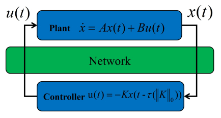
In practice, network operators tend to choose sparse communication topologies to cut costs, and the concurrent use of a communication network by multiple users commonly results in feedback delays. Our goal was to obtain the optimal sparse feedback control matrix $ K $. For this, we proposed a sparse optimal control (SOC) problem governed by the cyber-physical system with varying delay, to minimize $ ||K||_0 $ subject to a maximum allowable compromise in system cost. A penalty method was utilized to transform the SOC problem into a form that was constrained solely by box constraints. A smoothing technique was used to approximate the nonsmooth element in the resulting problem, and an analysis of the errors introduced by this technique was subsequently conducted. The gradients of the objective function concerning the feedback control matrix were obtained by solving the state system and a variational system simultaneously forward in time. An optimization algorithm was devised to tackle the resulting problem, building on the piecewise quadratic approximation. Finally, we have presented of simulations.
- cyber-physical system,
- $ l_0 $-norm of a matrix,
- sparse feedback matrix,
- varying delay,
- smoothing technique
Citation: Sida Lin, Dongyao Yang, Jinlong Yuan, Changzhi Wu, Tao Zhou, An Li, Chuanye Gu, Jun Xie, Kuikui Gao. A new computational method for sparse optimal control of cyber-physical systems with varying delay[J]. Electronic Research Archive, 2024, 32(12): 6553-6577. doi: 10.3934/era.2024306

Related Papers:

Abstract

In practice, network operators tend to choose sparse communication topologies to cut costs, and the concurrent use of a communication network by multiple users commonly results in feedback delays. Our goal was to obtain the optimal sparse feedback control matrix $ K $. For this, we proposed a sparse optimal control (SOC) problem governed by the cyber-physical system with varying delay, to minimize $ ||K||_0 $ subject to a maximum allowable compromise in system cost. A penalty method was utilized to transform the SOC problem into a form that was constrained solely by box constraints. A smoothing technique was used to approximate the nonsmooth element in the resulting problem, and an analysis of the errors introduced by this technique was subsequently conducted. The gradients of the objective function concerning the feedback control matrix were obtained by solving the state system and a variational system simultaneously forward in time. An optimization algorithm was devised to tackle the resulting problem, building on the piecewise quadratic approximation. Finally, we have presented of simulations.

References

[1]	M. Alowaidi, S. K. Sharma, A. AlEnizi, S. Bhardwaj, Integrating artificial intelligence in cyber security for cyber-physical systems, Electron. Res. Arch., 31 (2023), 1876–1896. http://doi.org/10.3934/era.2023097 doi: 10.3934/era.2023097
[2]	N. Negi, A. Chakrabortty, Sparsity-promoting optimal control of cyber-physical systems over shared communication networks, Automatica, 122 (2020), 109217. http://doi.org/10.1016/j.automatica.2020.109217 doi: 10.1016/j.automatica.2020.109217
[3]	M. N. Al-Mhiqani, T. Alsboui, T. Al-Shehari, K. H. Abdulkareem, R. Ahmad, M. A. Mohammed, Insider threat detection in cyber-physical systems: a systematic literature review, Comput. Electr. Eng., 119 (2024), 109489. http://doi.org/10.1016/j.compeleceng.2024.109489 doi: 10.1016/j.compeleceng.2024.109489
[4]	S. Liu, X. Wang, B. Niu, X. Song, H. Wang, X. Zhao, Adaptive resilient output feedback control against unknown deception attacks for nonlinear cyber-physical systems, IEEE Trans. Circuits Syst. II: Express Briefs, 71 (2024). 3855–3859. http://doi.org/10.1109/TCSII.2024.3372413 doi: 10.1109/TCSII.2024.3372413
[5]	M. Zhao, W. Qin, J. Yang, G. Lu, Security control for cyber-physical systems under aperiodic denial-of-service attacks: A memory-event-triggered active approach, Neurocomputing, 600 (2024), 128159. http://doi.org/10.1016/j.neucom.2024.128159 doi: 10.1016/j.neucom.2024.128159
[6]	P. E. G. Silva, P. H. J. Nardelli, A. S. de Sena, H. Siljak, N. Nevaranta, N. Marchetti, et al., Semantic-functional communications in cyber-physical systems, IEEE Network, 38 (2024), 241–249. http://doi.org/10.1109/MNET.2023.3329192 doi: 10.1109/MNET.2023.3329192
[7]	L. M. Castiglione, E. C. Lupu, Which attacks lead to hazards combining safety and security analysis for cyber-physical systems, IEEE Trans. Dependable Secure Comput., 21 (2024), 2526–2540. http://doi.org/10.1109/TDSC.2023.3309778 doi: 10.1109/TDSC.2023.3309778
[8]	S. Das, P. Dey, D. Chatterjee, Almost sure detection of the presence of malicious components in cyber-physical systems, Automatica, 167 (2024), 111789. http://doi.org/10.1016/j.automatica.2024.111789 doi: 10.1016/j.automatica.2024.111789
[9]	C. Fioravanti, S. Panzieri, G. Oliva, Negativizability: a useful property for distributed state estimation and control in cyber-physical systems, Automatica, 157 (2023), 111240. http://doi.org/10.1016/j.automatica.2023.111240 doi: 10.1016/j.automatica.2023.111240
[10]	H. N. AlEisa, F. Alrowais, R. Allafi, N. S. Almalki, R. Faqih, R. Marzouk, et al., Transforming transportation: safe and secure vehicular communication and anomaly detection with intelligent cyber-physical system and deep learning, IEEE Trans. Consum. Electron., 70 (2024), 1736–1746. http://doi.org/10.1109/TCE.2023.3325827 doi: 10.1109/TCE.2023.3325827
[11]	L. Khoshnevisan, X. Liu, Resilient neural network-based control of nonlinear heterogeneous multi-agent systems: a cyber-physical system approach, Nonlinear Dyn., 111 (2023), 19171–19185. http://doi.org/10.1007/s11071-023-08840-w doi: 10.1007/s11071-023-08840-w
[12]	L. Chen, Y. Li, S. Tong, Robust adaptive control for nonlinear cyber‐physical systems with FDI attacks via attack estimation, Int. J. Robust Nonlinear Control, 33 (2023), 9299–9316. http://doi.org/10.1002/rnc.6851 doi: 10.1002/rnc.6851
[13]	G. Routray, R. M. Hegde, Sparsity-driven loudspeaker gain optimization for sound field reconstruction with spherical microphone array, Digital Signal Process., 154 (2024), 104688. http://doi.org/10.1016/j.dsp.2024.104688 doi: 10.1016/j.dsp.2024.104688
[14]	K. Zhou, Y. Wang, B. Qiao, J. Liu, M. Liu, Z. Yang, et al., Non-convex sparse regularization via convex optimization for blade tip timing, Mech. Syst. Signal Process., 222 (2025), 111764. http://doi.org/10.1016/j.ymssp.2024.111764 doi: 10.1016/j.ymssp.2024.111764
[15]	T. Zhang, F. Peng, X. Tang, R. Yan, R. Deng, S. Zhao, A sparse knowledge embedded configuration optimization method for robotic machining system toward improving machining quality, Rob. Comput-Integr. Manuf., 90 (2024), 102818. http://doi.org/10.1016/j.rcim.2024.102818 doi: 10.1016/j.rcim.2024.102818
[16]	J. Yuan, C. Wu, K. L. Teo, J. Xie, S. Wang, Computational method for feedback perimeter control of multiregion urban traffic networks with state-dependent delays, Transp. Res. Part C: Emerging Technol., 153 (2023), 104231. https://doi.org/10.1016/j.trc.2023.104231 doi: 10.1016/j.trc.2023.104231
[17]	J. Yuan, C. Wu, K. L. Teo, S. Zhao, L. Meng, Perimeter control with state-dependent delays: optimal control model and computational method, IEEE Trans. Intell. Transp. Syst., 23 (2022), 20614–20627. https://doi.org/10.1109/TITS.2022.3179729 doi: 10.1109/TITS.2022.3179729
[18]	C. Zhao, Z. Luo, N. Xiu, Some advances in theory and algorithms for sparse optimization, Oper. Res. Trans., 24 (2020), 1–24.
[19]	S. Dai, Variable selection in convex quantile regression: $L_{1}$-norm or $L_{0}$-norm regularization?, Eur. J. Oper. Res., 305 (2023), 338–355. http://doi.org/10.1016/j.ejor.2022.05.041 doi: 10.1016/j.ejor.2022.05.041
[20]	B. Hong, H. Qian, Z. Wang, Iterative hard thresholding algorithm-based detector for compressed OFDM-IM systems, IEEE Commun. Lett., 26 (2022), 2205–2209. http://doi.org/10.1109/LCOMM.2022.3187451 doi: 10.1109/LCOMM.2022.3187451
[21]	H. Liu, T. Wang, Z. Liu, Some modified fast iterative shrinkage thresholding algorithms with a new adaptive non-monotone stepsize strategy for nonsmooth and convex minimization problems, Comput. Optim. Appl., 83 (2022), 651–691. http://doi.org/10.1007/s10589-022-00396-6 doi: 10.1007/s10589-022-00396-6
[22]	B. Liu, K. Gong, L. Zhang, Convergence analysis of the augmented Lagrangian method for $l_{p}$-norm cone optimization problems with $p\geq2$, Numer. Algorithms, 2024 (2024). http://doi.org/10.1007/s11075-024-01912-x doi: 10.1007/s11075-024-01912-x
[23]	D. Han, D. Sun, L. Zhang, Linear rate convergence of the alternating direction method of multipliers for convex composite programming, Math. Oper. Res., 43 (2018), 622–637. https://doi.org/10.1287/moor.2017.0875 doi: 10.1287/moor.2017.0875
[24]	E. Hernández, P. Merino, Sparse optimal control of timoshenko's beam using a locking-free finite element approximation, Optim. Control Appl. Methods, 45 (2024), 1007–1029. https://doi.org/10.1002/oca.3085 doi: 10.1002/oca.3085
[25]	K. Ito, T. Ikeda, K. Kashima, Sparse optimal stochastic control, Automatica, 125 (2021), 109438. http://doi.org/10.1016/j.automatica.2020.109438 doi: 10.1016/j.automatica.2020.109438
[26]	F. Lejarza, M. Baldea, Economic model predictive control for robust optimal operation of sparse storage networks, Automatica, 125 (2021), 109346. http://doi.org/10.1016/j.automatica.2020.109346 doi: 10.1016/j.automatica.2020.109346
[27]	M. Liu, H. Zhu, F. Zhang, J. Wang, C. Zhou, Y. Lv, Model-based sparse optimal control of the hydrogen sulfide synthesis process for acidic wastewater sulfidation, J. Water Process Eng., 65 (2024), 105836. http://doi.org/10.1016/j.jwpe.2024.105836 doi: 10.1016/j.jwpe.2024.105836
[28]	J. Yuan, C. Wu, Z. Liu, S. Zhao, C. Yu, K. L. Teo, et al., Koopman modeling for optimal control of the perimeter of multi-region urban traffic networks, Appl. Math. Modell., 138 (2025), 115742. https://doi.org/10.1016/j.apm.2024.115742 doi: 10.1016/j.apm.2024.115742
[29]	Q. Li, Y. Bai, C. Yu, Y. Yuan, A new piecewise quadratic approximation approach for $L_{0}$ norm minimization problem, Sci. China Math. 62 (2019), 185–204. http://doi.org/10.1007/s11425-017-9315-9 doi: 10.1007/s11425-017-9315-9
[30]	A. Modi, M. K. S. Faradonbeh, A. Tewari, G. Michailidis, Joint learning of linear time-invariant dynamical systems, Automatica, 164 (2024), 111635. http://doi.org/10.1016/j.automatica.2024.111635 doi: 10.1016/j.automatica.2024.111635
[31]	K. L. Teo, B. Li, C. Yu, V. Rehbock, Applied and Computational Optimal Control: a Control Parametrization Approach, Springer, Cham, 2021. http://doi.org/10.1007/978-3-030-69913-0
[32]	X. Wu, K. Zhang, M. Chen, A gradient-based algorithm for non-smooth constrained optimization problems governed by discrete-time nonlinear equations with application to long-term hydrothermal optimal scheduling control, J. Comput. Appl. Math., 412 (2022), 114335. https://doi.org/10.1016/j.cam.2022.114335 doi: 10.1016/j.cam.2022.114335

Reader Comments

Your name:*

Email:*
© 2024 the Author(s), licensee AIMS Press. This is an open access article distributed under the terms of the Creative Commons Attribution License (http://creativecommons.org/licenses/by/4.0)