Learning cooperative strategies in StarCraft through role-based monotonic value function factorization

Kun Han; Feng Jiang; Haiqi Zhu; Mengxuan Shao; Ruyu Yan; Kun Han; Feng Jiang; Haiqi Zhu; Mengxuan Shao; Ruyu Yan

doi:10.3934/era.2024037

Electronic Research Archive

2024, Volume 32, Issue 2: 779-798. doi: 10.3934/era.2024037

Previous Article Next Article

Research article Special Issues

Learning cooperative strategies in StarCraft through role-based monotonic value function factorization

1.
Faculty of Computing, Harbin Institute of Technology, Harbin 150000, China
2.
School of Medicine and Health, Harbin Institute of Technology, Harbin 150000, China
3.
School of Management, Harbin Institute of Technology, Harbin 150000, China

Received: 12 November 2023 Revised: 13 December 2023 Accepted: 02 January 2024 Published: 11 January 2024

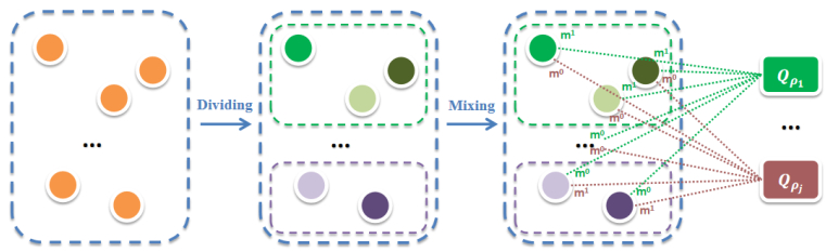
StarCraft is a popular real-time strategy game that has been widely used as a research platform for artificial intelligence. Micromanagement refers to the process of making each unit perform appropriate actions separately, depending on the current state in the the multi-agent system comprising all of the units, i.e., the fine-grained control of individual units for common benefit. Therefore, cooperation between different units is crucially important to improve the joint strategy. We have selected multi-agent deep reinforcement learning to tackle the problem of micromanagement. In this paper, we propose a method for learning cooperative strategies in StarCraft based on role-based montonic value function factorization (RoMIX). RoMIX learns roles based on the potential impact of each agent on the multi-agent task; it then represents the action value of a role in a mixed way based on monotonic value function factorization. The final value is calculated by accumulating the action value of all roles. The role-based learning improves the cooperation between agents on the team, allowing them to learn the joint strategy more quickly and efficiently. In addition, RoMIX can also reduce storage resources to a certain extent. Experiments show that RoMIX can not only solve easy tasks, but it can also learn better cooperation strategies for more complex and difficult tasks.
- Q-learning,
- multi-agent reinforcement learning,
- machine learning,
- artificial intelligence,
- StarCraft multi-agent challenge
Citation: Kun Han, Feng Jiang, Haiqi Zhu, Mengxuan Shao, Ruyu Yan. Learning cooperative strategies in StarCraft through role-based monotonic value function factorization[J]. Electronic Research Archive, 2024, 32(2): 779-798. doi: 10.3934/era.2024037

Related Papers:

Abstract

StarCraft is a popular real-time strategy game that has been widely used as a research platform for artificial intelligence. Micromanagement refers to the process of making each unit perform appropriate actions separately, depending on the current state in the the multi-agent system comprising all of the units, i.e., the fine-grained control of individual units for common benefit. Therefore, cooperation between different units is crucially important to improve the joint strategy. We have selected multi-agent deep reinforcement learning to tackle the problem of micromanagement. In this paper, we propose a method for learning cooperative strategies in StarCraft based on role-based montonic value function factorization (RoMIX). RoMIX learns roles based on the potential impact of each agent on the multi-agent task; it then represents the action value of a role in a mixed way based on monotonic value function factorization. The final value is calculated by accumulating the action value of all roles. The role-based learning improves the cooperation between agents on the team, allowing them to learn the joint strategy more quickly and efficiently. In addition, RoMIX can also reduce storage resources to a certain extent. Experiments show that RoMIX can not only solve easy tasks, but it can also learn better cooperation strategies for more complex and difficult tasks.

References

[1]	O. Vinyals, I. Babuschkin, W. M. Czarnecki, M. Mathieu, A. Dudzik, J. Chung, et al., Grandmaster level in StarCraft Ⅱ using multi-agent reinforcement learning, Nature, 575 (2019), 350–354. https://doi.org/10.1038/s41586-019-1724-z doi: 10.1038/s41586-019-1724-z
[2]	M. Samvelyan, T. Rashid, C. S. De Witt, G. Farquhar, N. Nardelli, T. G. Rudner, et al., The starcraft multi-agent challenge, preprint, arXiv: 1902.04043.
[3]	W. Huang, Q. Yin, J. Zhang, K. Huang, Learning Macromanagement in Starcraft by Deep Reinforcement Learning, Sensors, 21 (2021), 3332. https://doi.org/10.3390/s21103332 doi: 10.3390/s21103332
[4]	M. Kim, J. Oh, Y. Lee, J. Kim, S. Kim, S. Chong, et al., The StarCraft multi-agent exploration challenges: Learning multi-stage tasks and environmental factors without precise reward functions, IEEE Access, 11 (2023), 37854–37868. http://doi.org/10.1109/ACCESS.2023.3266652 doi: 10.1109/ACCESS.2023.3266652
[5]	A. Dafoe, E. Hughes, Y. Bachrach, T. Collins, K. R. McKee, J. Z. Leibo, et al., Open problems in cooperative AI, preprint, arXiv: 2012.08630.
[6]	Y. Zhang, Z. Mou, F. Gao, J. Jiang, R. Ding, Z. Han, UAV-enabled secure communications by multi-agent deep reinforcement learning, IEEE Trans. Veh. Technol., 69 (2020), 11599–11611. http://doi.org/10.1109/TVT.2020.3014788 doi: 10.1109/TVT.2020.3014788
[7]	A. Feriani, E. Hossain, Single and multi-agent deep reinforcement learning for AI-enabled wireless networks: A tutorial, IEEE Commun. Surv. Tutorials, 23 (2021), 1226–1252. http://doi.org/10.1109/COMST.2021.3063822 doi: 10.1109/COMST.2021.3063822
[8]	Z. Yan, Y. Xu, A multi-agent deep reinforcement learning method for cooperative load frequency control of a multi-area power system, IEEE Trans. Power Syst., 35 (2020), 4599–4608. http://doi.org/10.1109/TPWRS.2020.2999890 doi: 10.1109/TPWRS.2020.2999890
[9]	T. Wu, P. Zhou, K. Liu, Y. Yuan, X. Wang, H. Huang, et al., Multi-agent deep reinforcement learning for urban traffic light control in vehicular networks, IEEE Trans. Veh. Technol., 69 (2020), 8243–8256. http://doi.org/10.1109/TVT.2020.2997896 doi: 10.1109/TVT.2020.2997896
[10]	P. Hernandez-Leal, B. Kartal, M. E. Taylor, A survey and critique of multiagent deep reinforcement learning, Auton. Agent. Multi-Agent Syst., 33 (2019), 750–797. https://doi.org/10.1007/s10458-019-09421-1 doi: 10.1007/s10458-019-09421-1
[11]	T. T. Nguyen, N. D. Nguyen, S. Nahavandi, Deep reinforcement learning for multiagent systems: A Review of challenges, solutions, and applications, IEEE Trans. Cybern., 50 (2020), 3826–3839. https://doi.org/10.1109/TCYB.2020.2977374 doi: 10.1109/TCYB.2020.2977374
[12]	J. Foerster, G. Farquhar, T. Afouras, N. Nardelli, S. Whiteson, Counterfactual multi-agent policy gradients, in Thirty-Second AAAI Conference on Artificial Intelligence, 32 (2018), 2974–2982. https://doi.org/10.1609/aaai.v32i1.11794
[13]	C. Yu, A. Velu, E. Vinitsky, J. Gao, Y. Wang, A. Bayen, et al., The surprising effectiveness of PPO in cooperative multi-agent games, preprint, arXiv: 2103.01955.
[14]	P. Sunehag, G. Lever, A. Gruslys, W. M. Czarnecki, V. Zambaldi, M. Jaderberg, et al., Value-decomposition networks for cooperative multi-agent learning, preprint, arXiv: 1706.05296.
[15]	T. Rashid, M. Samvelyan, C. S. De Witt, G. Farquhar, J. Foerster, S. Whiteson, Monotonic value function factorisation for deep multi-agent reinforcement learning, preprint, arXiv: 1803.11485.
[16]	C. Claus, C. Boutilier, The dynamics of reinforcement learning in cooperative multiagent systems, in Proceedings of the Fifteenth National Conference on Artificial Intelligence, (1998), 746–752.
[17]	M. Tan, Multi-agent reinforcement learning: Independent vs. cooperative agents, in Proceedings of the Tenth International Conference on Machine Learning, (1993), 330–337. https://doi.org/10.1016/B978-1-55860-307-3.50049-6
[18]	V. Mnih, K. Kavukcuoglu, D. Silver, A. Graves, I. Antonoglou, D. Wierstra, et al., Playing atari with deep reinforcement learning, preprint, arXiv: 1312.5602.
[19]	W. Qi, S. E. Ovur, Z. Li, A. Marzullo, R. Song, Multi-sensor guided hand gesture recognition for a teleoperated robot using a recurrent neural network, IEEE Robot. Autom. Lett., 6 (2021), 6039–6045. https://doi.org/10.1109/LRA.2021.3089999 doi: 10.1109/LRA.2021.3089999
[20]	W. Qi, A. Aliverti, A multimodal wearable system for continuous and real-time breathing pattern monitoring during daily activity, IEEE J. Biomed. Health Inf., 24 (2020), 2199–2207. https://doi.org/10.1109/JBHI.2019.2963048 doi: 10.1109/JBHI.2019.2963048
[21]	Q. Fu, T. Qiu, J. Yi, Z. Pu, S. Wu, Concentration network for reinforcement learning of large-scale multi-agent systems, in AAAI Technical Track on Multiagent Systems, (2022), 9341–9349. https://doi.org/10.1609/aaai.v36i9.21165
[22]	Y. Wang, C. W. De Silva, Multi-robot box-pushing: Single-agent Q-Learning vs. team Q-Learning, in 2006 IEEE/RSJ International Conference on Intelligent Robots and Systems, (2006), https://doi.org/10.1109/IROS.2006.281729
[23]	A. Galindo-Serrano, L. Giupponi, Distributed Q-learning for aggregated interference control in cognitive radio networks, IEEE Trans. Veh. Technol., 59 (2010), 1823–1834. http://doi.org/10.1109/TVT.2010.2043124 doi: 10.1109/TVT.2010.2043124
[24]	X. Wang, T, Sandholm, Reinforcement learning to play an optimal Nash equilibrium in team Markov games, in Advances in Neural Information Processing Systems, (2002).
[25]	G. Arslan, S. Yüksel, Decentralized Q-learning for stochastic teams and games, IEEE Trans. Autom. Control, 62 (2017), 1545–1558. http://doi.org/10.1109/TAC.2016.2598476 doi: 10.1109/TAC.2016.2598476
[26]	K. Son, D. Kim, W. J. Kang, D. E. Hostallero, Y. Yi, QTRAN: Learning to factorize with transformation for cooperative multi-agent reinforcement learning, in Proceedings of the 36th International Conference on Machine Learning, (2019), 5887–5896.
[27]	A. Mahajan, T. Rashid, M. Samvelyan, S.Whiteson, MAVEN: Multi-agent variational exploration, in 33rd Conference on Neural Information Processing Systems, (2019), 1–12.
[28]	Y. Yang, J. Hao, B. Liao, K. Shao, G. Chen, W. Liu, et al., Qatten: A general framework for cooperative multiagent reinforcement learning, preprint, arXiv: 2002.03939.
[29]	M. J. Khan, S. H. Ahmed, G. Sukthankar, Transformer-based value function decomposition for cooperative multi-agent reinforcement learning in StarCraft, in Eighteenth AAAI Conference on Artificial Intelligence and Interactive Digital Entertainment, 18 (2022), 113–119. https://doi.org/10.1609/aiide.v18i1.21954
[30]	C. Wu, F. Wu, T. Qi, Y. Huang, X. Xie, Fastformer: Additive attention can be all you need, preprint, arXiv: 2108.09084.
[31]	T. Rashid, G. Farquhar, B. Peng, S. Whiteson, Weighted QMIX: Expanding monotonic value function factorisation for deep multi-agent reinforcement learning, in 34th Conference on Neural Information Processing Systems, (2020), 1–12.
[32]	J. Wang, Z. Ren, T. Liu, Y. Yu, C. Zhang, QPLEX: Duplex dueling multi-agent Q-learning, preprint, arXiv: 2008.01062.
[33]	Z. Wang, T. Schaul, M. Hessel, H. Hasselt, M. Lanctot, N. Freitas, Dueling network architectures for deep reinforcement learning, in Proceedings of The 33rd International Conference on Machine Learning, (2016), 199–2003.
[34]	S. Iqbal, F. Sha, Actor-attention-critic for multi-agent reinforcement learning, in Proceedings of the 36th International Conference on Machine Learning, (2019), 2961–2970.
[35]	T. Zhang, H. Xu, X. Wang, Y. Wu, K. Keutzer, J. E. Gonzalez, et al., Multi-agent collaboration via reward attribution decomposition, preprint, arXiv: 2010.08531.
[36]	Y. Liu, W. Wang, Y. Hu, J. Hao, X. Chen, Y. Gao, Multi-agent game abstraction via graph attention neural network, in Proceedings of the AAAI Conference on Artificial Intelligence, 34 (2020), 7211–7218. https://doi.org/10.1609/aaai.v34i05.6211
[37]	T. Wang, T. Gupta, A. Mahajan, B. Peng, S. Whiteson, C. Zhang, RODE: Learning roles to decompose multi-agent tasks, preprint, arXiv: 2010.01523.
[38]	J. Zhao, Y. Lv, Output-feedback Robust Tracking Control of Uncertain Systems via Adaptive Learning, Int. J. Control Autom. Syst., 21 (2023), 1108–1118. https://doi.org/10.1007/s12555-021-0882-6 doi: 10.1007/s12555-021-0882-6
[39]	Y. Wang, Z. Liu, J. Xu, W. Yan, Heterogeneous network representation learning approach for ethereum identity identification, IEEE Trans. Comput. Soc. Syst., 10 (2023), 890–899. https://doi.org/10.1109/TCSS.2022.3164719 doi: 10.1109/TCSS.2022.3164719
[40]	F. A. Oliehoek, C. Amato, A Concise Introduction to Decentralized POMDPs, Springer, Cham, 2016. https://doi.org/10.1007/978-3-319-28929-8
[41]	M. Hausknecht, P. Stone, Deep recurrent Q-learning for partially observable MDPs, preprint, arXiv: 1507.06527.

Reader Comments

Your name:*

Email:*
© 2024 the Author(s), licensee AIMS Press. This is an open access article distributed under the terms of the Creative Commons Attribution License (http://creativecommons.org/licenses/by/4.0)