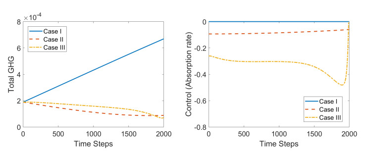
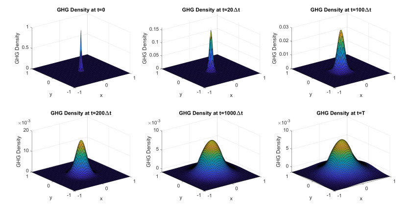
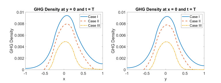
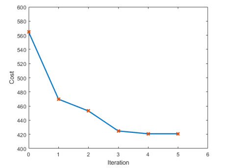
In this paper, we propose a space-time dynamic model for describing the temporal evolution of greenhouse gas concentration in the atmosphere. We use this dynamic model to develop an optimal control strategy for reduction of atmospheric pollutants. We prove the existence of optimal policies subject to control constraints. Further, we present necessary conditions of optimality using which one can determine such policies. A convergence theorem for computation of the optimal policies is also presented. Simulation results illustrate removal of greenhouse gas using the optimal policies.
Citation: N. U. Ahmed, Saroj Biswas. Optimal strategy for removal of greenhouse gas in the atmosphere to avert global climate crisis[J]. Electronic Research Archive, 2023, 31(12): 7452-7472. doi: 10.3934/era.2023376
In this paper, we propose a space-time dynamic model for describing the temporal evolution of greenhouse gas concentration in the atmosphere. We use this dynamic model to develop an optimal control strategy for reduction of atmospheric pollutants. We prove the existence of optimal policies subject to control constraints. Further, we present necessary conditions of optimality using which one can determine such policies. A convergence theorem for computation of the optimal policies is also presented. Simulation results illustrate removal of greenhouse gas using the optimal policies.

| [1] | Intergovernmental Panel on Climate Change (IPCC), Climate Change 2022: Mitigation of Climate Change, Cambridge University Press, 2023. https://doi.org/10.1017/9781009157926 |
| [2] | EPA, Overview of Greenhouse Gases, 2023. Available from: https://www.epa.gov/ghgemissions/overview-greenhouse-gases. |
| [3] | EPA, Sources of Greenhouse Gas Emissions, 2023. Available from: https://www.epa.gov/ghgemissions/sources-greenhouse-gas-emissions. |
| [4] |
S. Soldatenko, A. Bogomolov, A. Ronzhin, Mathematical modeling of climate change and variability in the context of outdoor ergonomics, Mathematics, 9 (2021), 2920. https://doi.org/10.3390/math9222920 doi: 10.3390/math9222920

|
| [5] |
N. Jeevanjee, P. Hassanzadeh, S. Hill, A. Sheshadri, A perspective on climate model hierarchies, J. Adv. Model. Earth Syst., 9 (2017), 1760–1771. https://doi.org/10.1002/2017MS001038 doi: 10.1002/2017MS001038
|
| [6] |
P. Maher, E. Gerber, B. Medeiros, T. Merlis, S. Sherwood, A. Sheshadri, et al., Model hierarchies for understanding atmospheric circulation, Rev. Geophys., 57 (2019), 250–280. https://doi.org/10.1029/2018RG000607 doi: 10.1029/2018RG000607
|
| [7] |
K. Tung, Simple climate modeling, Discrete Contin. Dyn. Syst. - Ser. B, 7 (2007), 651–660. https://doi.org/10.3934/dcdsb.2007.7.651 doi: 10.3934/dcdsb.2007.7.651
|
| [8] |
J. Murphy, D. Sexton, D. Barnett, G. Jones, M. Webb, M. Collins, et al., Quantification of modelling uncertainties in a large ensemble of climate change simulations, Nature, 430 (2004), 768–772. https://doi.org/10.1038/nature02771 doi: 10.1038/nature02771
|
| [9] |
S. Bony, R. Colman, V. Kattsov, R. Allan, C. Bretherton, J. L. Dufresne, et al., How well do we understand and evaluate climate change feedback processes, J. Clim., 19 (2006), 3445–3482. https://doi.org/10.1175/JCLI3819.1 doi: 10.1175/JCLI3819.1
|
| [10] |
C. Li, Quantifying greenhouse gas emissions from soils: Scientific basis and modeling approach, Soil Sci. Plant Nutr., 53 (2007), 344–352. https://doi.org/10.1111/j.1747-0765.2007.00133.x doi: 10.1111/j.1747-0765.2007.00133.x
|
| [11] |
C. Rotz, Symposium review: Modeling greenhouse gas emissions from dairy farms, J. Dairy Sci., 101 (2018), 6675–6690. https://doi.org/10.3168/jds.2017-13272 doi: 10.3168/jds.2017-13272
|
| [12] | S. Khan, N. U. Ahmed, An attempt towards dynamic modeling of the earth's climate system, Dyn. Syst. Appl., 24 (2015), 155–168. |
| [13] |
G. Q. Sun, L. Li, J. Li, C. Liu, Y. P. Wu, S. Gao, et al., Impacts of climate change on vegetation pattern: Mathematical modeling and data analysis, Phys. Life Rev., 43 (2022), 239–270. https://doi.org/10.1016/j.plrev.2022.09.005 doi: 10.1016/j.plrev.2022.09.005
|
| [14] |
T. Smith, H. Shugart, G. Bonan, J. Smith, Modeling the potential response of vegetation to global climate change, Adv. Ecol. Res., 22 (1992), 93–116. https://doi.org/10.1016/S0065-2504(08)60134-8 doi: 10.1016/S0065-2504(08)60134-8
|
| [15] |
S. Scheiter, S. Higgins, Impacts of climate change on the vegetation of Africa: An adaptive dynamic vegetation modelling approach, Global Change Biol., 15 (2009), 2224–2246. https://doi.org/10.1111/j.1365-2486.2008.01838.x doi: 10.1111/j.1365-2486.2008.01838.x
|
| [16] |
S. Kefi, M. Rietkerk, G. Katul, Vegetation pattern shift as a result of rising atmospheric CO$_2$ in arid ecosystems, Theor. Popul. Biol., 74 (2008), 332–344. https://doi.org/10.1016/j.tpb.2008.09.004 doi: 10.1016/j.tpb.2008.09.004
|
| [17] |
J. Rombouts, M. Ghil, Oscillations in a simple climate–vegetation model, Nonlinear Processes Geophys., 22 (2015), 275–288. https://doi.org/10.5194/npg-22-275-2015 doi: 10.5194/npg-22-275-2015
|
| [18] |
C. Klausmeier, Regular and irregular patterns in semiarid vegetation, Science, 284 (1999), 1826–1828. https://doi.org/10.1126/science.284.5421.1826 doi: 10.1126/science.284.5421.1826
|
| [19] |
J. Liang, C. Liu, G. Q. Sun, L. Li, L. Zhang, M. Hou, et al., Nonlocal interactions between vegetation induce spatial patterning, Appl. Math. Comput., 428 (2022), 127061. https://doi.org/10.1016/j.amc.2022.127061 doi: 10.1016/j.amc.2022.127061
|
| [20] |
C. Murphy, A. Coen, I. Clancy, V. Decristoforo, S. Cathal, K. Healion, et al., The emergence of a climate change signal in long-term Irish meteorological observations, Weather Clim. Extremes, 42 (2023), 100608. https://doi.org/10.1016/j.wace.2023.100608 doi: 10.1016/j.wace.2023.100608
|
| [21] |
R. Wang, J. Zhang, C. Cai, H. Zhang, How to control Nitrogen and Phosphorus loss during runoff process? – A case study at Fushi Reservoir in Anji County (China), Ecol. Indic., 155 (2023), 111007. https://doi.org/10.1016/j.ecolind.2023.111007 doi: 10.1016/j.ecolind.2023.111007
|
| [22] | EPA, GHG Reduction Programs and Strategies, 2023. Available from: https://www.epa.gov/climateleadership/ghg-reduction-programs-strategies. |
| [23] | European Environment Agency, Climate change mitigation: reducing emissions, 2023. Available from: https://www.eea.europa.eu/en/topics/in-depth/climate-change-mitigation-reducing-emissions. |
| [24] | London School of Economics and Political Science, What is carbon capture, usage and storage (CCUS) and what role can it play in tackling climate change, 2023. Available from: https://www.lse.ac.uk/granthaminstitute/explainers/what-is-carbon-capture-and-storage-and-what-role-can-it-play-in-tackling-climate-change/. |
| [25] | International Energy Agency, Carbon Capture, Utilization and Storage, 2023. Available from: https://www.iea.org/energy-system/carbon-capture-utilisation-and-storage. |
| [26] | N. U. Ahmed, K. L. Teo, Optimal Control of Distributed Parameter Systems, Elsevier Science Inc., North Holland, New York, USA, 1981. |
| [27] | J. L. Lions, Optimal Control of Systems Governed by Partial Differential Equations, Springer Verlag, Berlin · Heidelberg, Germany, 1971. |

Figures(5)
N. U. Ahmed, Saroj Biswas. Optimal strategy for removal of greenhouse gas in the atmosphere to avert global climate crisis[J]. Electronic Research Archive, 2023, 31(12): 7452-7472. doi: 10.3934/era.2023376


 DownLoad: