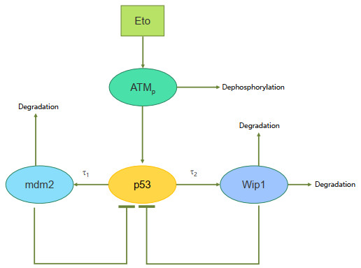
In this paper, the kinetics of p53 in two cell lines with different degrees of sensitivity to chemotherapeutic drugs is studied. There is much research that has explored the p53 oscillation, but there are few comparisons between cells that are sensitive to drug treatment and those that are not. Here, the kinetics of the p53 system between etoposide-sensitive and etoposide-resistant cell lines in response to different drug doses and different protein synthesis time delays are studied and compared. First, the results showed that time delay is an important condition for p53 oscillation by producing Hopf bifurcation in both the etoposide-sensitive and etoposide-resistant cells. If the protein synthesis time delays are zero, the system cannot oscillate even the dose of the drug increases. Second, the time delay required for producing sustained oscillation in sensitive cells is shorter than the drug-resistant cells. In addition, the p53-Wip1 negative feedback loop in drug-resistant cells is relatively highly strengthened than the drug-sensitive cells. To sum up, p53 oscillation is controlled by time delay, drug dose, and the coupled negative feedback network including p53-mdm2 and p53-wip1. Moreover, in the two different types of cells, the control mechanisms are similar, but there are also differences.
Citation: Fang Yan, Changyong Dai, Haihong Liu. Oscillatory dynamics of p53 pathway in etoposide sensitive and resistant cell lines[J]. Electronic Research Archive, 2022, 30(6): 2075-2108. doi: 10.3934/era.2022105
In this paper, the kinetics of p53 in two cell lines with different degrees of sensitivity to chemotherapeutic drugs is studied. There is much research that has explored the p53 oscillation, but there are few comparisons between cells that are sensitive to drug treatment and those that are not. Here, the kinetics of the p53 system between etoposide-sensitive and etoposide-resistant cell lines in response to different drug doses and different protein synthesis time delays are studied and compared. First, the results showed that time delay is an important condition for p53 oscillation by producing Hopf bifurcation in both the etoposide-sensitive and etoposide-resistant cells. If the protein synthesis time delays are zero, the system cannot oscillate even the dose of the drug increases. Second, the time delay required for producing sustained oscillation in sensitive cells is shorter than the drug-resistant cells. In addition, the p53-Wip1 negative feedback loop in drug-resistant cells is relatively highly strengthened than the drug-sensitive cells. To sum up, p53 oscillation is controlled by time delay, drug dose, and the coupled negative feedback network including p53-mdm2 and p53-wip1. Moreover, in the two different types of cells, the control mechanisms are similar, but there are also differences.

| [1] |
K. Vahakangas, Molecular Epidemiology of Human Cancer Risk, Lung Cancer, 2003, 43–59. https://doi.org/10.1385/1-59259-323-2:43 doi: 10.1385/1-59259-323-2:43

|
| [2] |
F. Murray-Zmijewski, E. A. Slee, X. Lu, A complex barcode underlies the heterogeneous response of p53 to stress, Nat. Rev. Mol. Cell Biol., 9 (2008), 702–712. https://doi.org/10.1038/nrm2451 doi: 10.1038/nrm2451
|
| [3] |
K. H. Vousden, Outcomes of p53 activation-spoilt for choice, J. Cell Sci., 119 (2006), 5015–5020. https://doi.org/10.1242/jcs.03293 doi: 10.1242/jcs.03293
|
| [4] |
X. P. Zhang, F. Liu, Z, Cheng, W. Wang, Cell fate decision mediated by p53 pulses, Proc. Natl. Acad. Sci. U.S.A., 106 (2009), 12245–12250. https://doi.org/10.1073/pnas.0813088106 doi: 10.1073/pnas.0813088106
|
| [5] |
X. P. Zhang, F. Liu, W. Wang, Two-phase dynamics of p53 in the DNA damage response, Proc. Natl. Acad. Sci. U.S.A., 108 (2011), 8990–8995. https://doi.org/10.1073/pnas.1100600108 doi: 10.1073/pnas.1100600108
|
| [6] |
K. H. Vousden, D. P. Lane, p53 in health and disease, Nat. Rev. Mol. Cell Biol., 8 (2007), 275–283. https://doi.org/10.1038/nrm2147 doi: 10.1038/nrm2147
|
| [7] |
S. Shangary, S. Wang, Small-molecule inhibitors of the MDM2-p53 protein-protein interaction to reactivate p53 function: a novel approach for cancer therapy, Annu. Rev. Pharmacol., 49 (2009), 223–241. https://doi.org/10.1146/annurev.pharmtox.48.113006.094723 doi: 10.1146/annurev.pharmtox.48.113006.094723
|
| [8] |
M. J. Duffy, N. C. Synnott, J. Crown, Mutant p53 as a target for cancer treatment, Eur. J. Cancer., 83 (2017), 258–265. https://doi.org/10.1016/j.ejca.2017.06.023 doi: 10.1016/j.ejca.2017.06.023
|
| [9] |
V. J. N. Bykov, S. E. Eriksson, J. Bianchi, K. G. Wiman, Targeting mutant p53 for efficient cancer therapy, Nat. Rev. Cancer., 18 (2018), 89–102. https://doi.org/10.1038/nrc.2017.109 doi: 10.1038/nrc.2017.109
|
| [10] |
Y. Pan, Y. Yuan, G. Liu, Y. Wei, P53 and Ki-67 as prognostic markers in triple-negative breast cancer patients, Plos One, 12 (2017), e0172324. https://doi.org/10.1371/journal.pone.0172324 doi: 10.1371/journal.pone.0172324
|
| [11] |
D. Michael, M. Oren, The p53-Mdm2 module and the ubiquitin system, Semin. Cancer Biol., 13 (2003), 49–58. https://doi.org/10.1016/S1044-579X(02)00099-8 doi: 10.1016/S1044-579X(02)00099-8
|
| [12] |
Y. Haupt, R. Maya, A. Kazaz, M. Oren, Mdm2 promotes the rapid degradation of p53, Nature, 387 (1997), 296–299. https://doi.org/10.1038/387296a0 doi: 10.1038/387296a0
|
| [13] |
L. Ma, J. Wagner, J. J. Rice, W. Hu, A. J. Levine, G. A. Stolovitzky, A plausible model for the digital response of p53 to DNA damage, Proc. Natl. Acad. Sci. U.S.A., 102 (2005), 14266–14271. https://doi.org/10.1073/pnas.0501352102 doi: 10.1073/pnas.0501352102
|
| [14] |
R. L. Bar-Or, R, Maya, L. A. Segel, U. Alon, A. J. Levine, M. Oren, Generation of oscillations by the p53-Mdm2 feedback loop: a theoretical and experimental study, Proc. Natl. Acad. Sci. U.S.A., 97 (2000), 11250–11255. https://doi.org/10.1073/pnas.210171597 doi: 10.1073/pnas.210171597
|
| [15] |
J. H. Park, S. W. Yang, J. M. Park, S. H. Ka, J. Kim, Y. Kong, et al., Positive feedback regulation of p53 transactivity by DNA damage-induced ISG15 modification, Nat. Commun., 7 (2016), 12513. https://doi.org/10.1038/ncomms12513 doi: 10.1038/ncomms12513
|
| [16] |
H. Cha, J. M. Lowe, H. Li, J. Lee, G. I. Belova, D. V. Bulavin, et al., Wip1 directly dephosphorylates $\gamma$-H2AX and attenuates the DNA damage response, Cancer Res., 70 (2010), 4112–4122. https://doi.org/10.1158/0008-5472.CAN-09-4244 doi: 10.1158/0008-5472.CAN-09-4244
|
| [17] |
H. Sakai, H. Fujigaki, S. Mazur, E. Appella, Wild-type p53-induced phosphatase 1 (Wip1) forestalls cellular premature senescence at physiological oxygen levels by regulating DNA damage response signaling during DNA replication, Cell Cycle, 13 (2014), 1015–1029. https://doi.org/10.4161/cc.27920 doi: 10.4161/cc.27920
|
| [18] |
S. Shreeram, O. N. Demidov, W. K. Hee, H. Yamaguchi, N. Onishi, C. Kek, et al., Wip1 phosphatase modulates ATM-dependent signaling pathways, Mol. Cell, 23 (2006), 757–764. https://doi.org/10.1016/j.molcel.2006.07.010 doi: 10.1016/j.molcel.2006.07.010
|
| [19] |
N. Geva-Zatorsky, N. Rosenfeld, S. Itzkovitz, R. Milo, A. Sigal, E. Dekel, et al., Oscillations and variability in the p53 system, Mol. Syst. Biol., 2 (2006), 0033. https://doi.org/10.1038/msb4100068 doi: 10.1038/msb4100068
|
| [20] |
A. M. Weber, A. J. Ryan, ATM and ATR as therapeutic targets in cancer, Pharmacol. Ther., 149 (2015), 124–138. https://doi.org/10.1016/j.pharmthera.2014.12.001 doi: 10.1016/j.pharmthera.2014.12.001
|
| [21] |
S. Banin, L. Moyal, S. Shieh, Y. Taya, C. W. Anderson, L. Chessa, et al., Enhanced phosphorylation of p53 by ATM in response to DNA damage, Science, 281 (1998), 1674–1677. https://doi.org/10.1126/science.281.5383.1674 doi: 10.1126/science.281.5383.1674
|
| [22] |
E. Haines, A. Zimmermann, F. Zenke, A. Blaukat, Selective DNA-PK inhibitor, M3814, boosts p53 apoptotic response to DNA double strand breaks and effectively kills acute leukemia cell: Implications for AML therapy, Cancer Res., 78 (2018), 4830–4830. https://doi.org/10.1158/1538-7445.AM2018-4830 doi: 10.1158/1538-7445.AM2018-4830
|
| [23] |
W. Freed-Pastor, C. Prives, Targeting mutant p53 through the mevalonate pathway, Nat. Cell Biol., 18 (2016), 1122–1124. https://doi.org/10.1038/ncb3435 doi: 10.1038/ncb3435
|
| [24] |
R. J. Ihry, K. A. Worringer, M. R. Salick, E. Frias, D. Ho, K. Theriault, et. al., p53 inhibits CRISPR–Cas9 engineering in human pluripotent stem cell, Nat. Med., 24 (2018), 939–946. https://doi.org/10.1101/168443 doi: 10.1101/168443
|
| [25] |
Q. Cheng, J. Chen, Mechanism of p53 stabilization by ATM after DNA damage, Cell Cycle, 9 (2010), 472–478. https://doi.org/10.4161/cc.9.3.10556 doi: 10.4161/cc.9.3.10556
|
| [26] |
C. Zhou, X. Zhang, F. Liu, W. Wang, Modeling the interplay between the HIF-1 and p53 pathways in hypoxia, Sci. Rep., 5 (2015), 13834. https://doi.org/10.1038/srep13834 doi: 10.1038/srep13834
|
| [27] |
X. Tian, B. Huang, X. Zhang, M. Liu, F. Liu, J. N. Onuchic, W. Wang, Modeling the response of a tumor-suppressive network to mitogenic and oncogenic signals, Proc. Natl. Acad. Sci. U.S.A., 114 (2017), 5337–5342. https://doi.org/10.1073/pnas.1702412114 doi: 10.1073/pnas.1702412114
|
| [28] |
D. Bratsun, D. Volfson, L. S. Tsimring, J. Hasty, Delay-induced stochastic oscillations in gene regulation, Proc. Natl. Acad. Sci. U.S.A., 102 (2005), 14593–14598. https://doi.org/10.1073/pnas.0503858102 doi: 10.1073/pnas.0503858102
|
| [29] |
B. Novák, J. J. Tyson, Design principles of biochemical oscillators, Nat. Rev. Mol. Cell Biol., 9 (2008), 981–991. https://doi.org/10.1038/nrm2530 doi: 10.1038/nrm2530
|
| [30] |
A. Honkela, J. Peltonen, H. Topa, I. Charapitsa, F. Matarese, K. Grote, et al., Genome-wide modeling of transcription kinetics reveals patterns of RNA production delays, Proc. Natl. Acad. Sci. U.S.A., 112 (2015), 13115–13120. https://doi.org/10.1073/pnas.1420404112 doi: 10.1073/pnas.1420404112
|
| [31] |
A. Prindle, J. Selimkhanov, H. Li, I. Razinkov, L. S. Tsimring, J. Hasty, Rapid and tunable post-translational coupling of genetic circuits, Nature, 508 (2014), 387–391. https://doi.org/10.1038/nature13238 doi: 10.1038/nature13238
|
| [32] |
H. K. Yalamanchili, B. Yan, J. Li, J. Qin, Z. Zhao, F. Y. L. Chin, et al., DDGni: dynamic delay gene-network inference from high-temporal data using gapped local alignment, Bioinformatics, 30 (2013), 377–383. https://doi.org/10.1093/bioinformatics/btt692 doi: 10.1093/bioinformatics/btt692
|
| [33] |
R. Yang, B. Huang, Y. Zhu, Y. Li, F. Liu, J. Shi, Cell type-dependent bimodal p53 activation engenders a dynamic mechanism of chemoresistance, Sci. Adv., 4 (2018), eaat5077. https://doi.org/10.1126/sciadv.aat5077 doi: 10.1126/sciadv.aat5077
|
| [34] |
C. Prives, Signaling to p53: breaking the MDM2–p53 circuit, Cell, 95 (1998), 5–8. https://doi.org/10.1016/S0092-8674(00)81774-2 doi: 10.1016/S0092-8674(00)81774-2
|
| [35] |
J. M. Stommel, G. M. Wahl, Accelerated MDM2 auto-degradation induced by DNA-damage kinases is required for p53 activation, The EMBO J., 23 (2004), 1547–1556. https://doi.org/10.1038/sj.emboj.7600145 doi: 10.1038/sj.emboj.7600145
|
| [36] |
E. Batchelor, C. S. Mock, I. Bhan, A. Loewer, G. Lahav, Recurrent initiation: a mechanism for triggering p53 pulses in response to DNA damage, Mol. cell., 30 (2008), 277–289. https://doi.org/10.1016/j.molcel.2008.03.016 doi: 10.1016/j.molcel.2008.03.016
|
| [37] |
N. A. M. Monk, Oscillatory expression of Hes1, p53, and NF-kappaB driven by transcriptional time delays, Curr. Biol., 13 (2003), 1409–1413. https://doi.org/10.1016/S0960-9822(03)00494-9 doi: 10.1016/S0960-9822(03)00494-9
|
| [38] |
Y. Zhang, H. Liu, F. Yan, J. Zhou, Oscillatory dynamics of p38 activity with transcriptional and translational time delays, Sci. Rep., 7 (2017), 11495. https://doi.org/10.1038/s41598-017-11149-5 doi: 10.1038/s41598-017-11149-5
|
| [39] |
D. M. Longo, J. Selimkhanov, J. D. Kearns, J. Hasty, A. Hoffmann, L. S. Tsimring, Dual Delayed Feedback Provides Sensitivity and Robustness to the NF-$\kappa$B Signaling Module, PLoS Comput. Biol., 9 (2013), e1003112. https://doi.org/10.1371/journal.pcbi.1003112 doi: 10.1371/journal.pcbi.1003112
|
| [40] |
Q. Wang, M. Perc, Z. Duan, G. Chen, Synchronization transitions on scale-free neuronal networks due to finite information transmission delays, Phys. Rev. E., 80 (2009), 026206. https://doi.org/10.1103/PhysRevE.80.026206 doi: 10.1103/PhysRevE.80.026206
|
| [41] |
Q. Wang, H. Zhang, G. Chen, Stimulus-induced transition of clustering firings in neuronal networks with information transmission delay, Eur. Phys. J. B., 86 (2013), 301. https://doi.org/10.1140/epjb/e2013-40078-3 doi: 10.1140/epjb/e2013-40078-3
|
| [42] |
A. Roxin, N. Brunel, D. Hansel, Role of delays in shaping spatiotemporal dynamics of neuronal activity in large networks, Phys. Rev. Lett., 94 (2005), 238103. https://doi.org/10.1103/PhysRevLett.94.238103 doi: 10.1103/PhysRevLett.94.238103
|
| [43] |
E. Rossoni, Y. Chen, M. Ding, J. Feng, Stability of synchronous oscillations in a system of Hodgkin-Huxley neurons with delayed diffusive and pulsed coupling, Phys. Rev. E., 71 (2005), 061904. https://doi.org/10.1103/PhysRevE.71.061904 doi: 10.1103/PhysRevE.71.061904
|
| [44] |
J. Lewis, Autoinhibition with transcriptional delay: A simple mechanism for the zebrafish somitogenesis oscillator, Curr. Biol. Cb., 13 (2003), 1398–1408. https://doi.org/10.1016/s0960-9822(03)00534-7 doi: 10.1016/s0960-9822(03)00534-7
|
| [45] |
A. Audibert, D. Weil, F. Dautry, In vivo kinetics of mRNA splicing and transport in mammalian cells, Mol. Cell. Biol., 22 (2002), 6706–6718. https://doi.org/10.1128/MCB.22.19.6706–6718.2002 doi: 10.1128/MCB.22.19.6706–6718.2002
|
| [46] | B. D. Hassard, N. D. Kazarinoff, Y. H. Wan, Theory and applications of Hopf bifurcation, Cambridge University Press, (1981). http://dx.doi.org/10.1090/conm/445 |


Figures(17) / Tables(2)
Fang Yan, Changyong Dai, Haihong Liu. Oscillatory dynamics of p53 pathway in etoposide sensitive and resistant cell lines[J]. Electronic Research Archive, 2022, 30(6): 2075-2108. doi: 10.3934/era.2022105


 DownLoad: