Firing activities and magnetic stimulation effects in a Cortico-basal ganglia-thalamus neural network

Zilu Cao; Lin Du; Honghui Zhang; Lianghui Qu; Luyao Yan; Zichen Deng; Zilu Cao; Lin Du; Honghui Zhang; Lianghui Qu; Luyao Yan; Zichen Deng

doi:10.3934/era.2022104

Electronic Research Archive

2022, Volume 30, Issue 6: 2054-2074. doi: 10.3934/era.2022104

Previous Article Next Article

Research article Special Issues

Firing activities and magnetic stimulation effects in a Cortico-basal ganglia-thalamus neural network

1.
School of Mathematics and Statistics, Northwestern Polytechnical University, 1 Dongxiang Road, Chang'an District, Xi'an, Shaanxi, 710129, China
2.
School of Aeronautics, Northwestern Polytechnical University, 127 West Youyi Road, Beilin District, Xi'an, Shaanxi, 710072, China
3.
College of Science, Zhongyuan University of Technology, No. 41 Zhongyuan Road (M), Zhengzhou, Henan, 450007, China
4.
MIIT Key Laboratory of Dynamics and Control of Complex Systems, 1 Dongxiang Road, Chang'an District, Xi'an, Shaanxi, 710129, China

Received: 28 September 2021 Revised: 29 November 2021 Accepted: 09 December 2021 Published: 14 April 2022

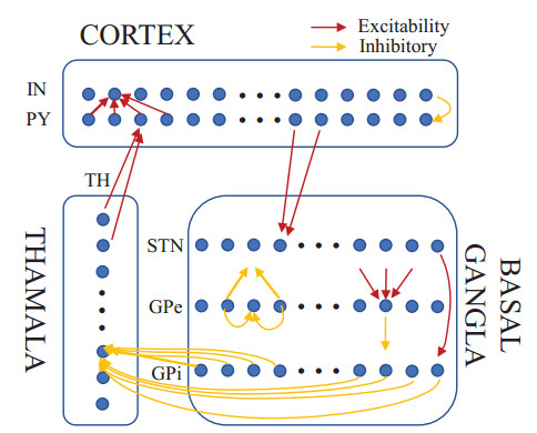
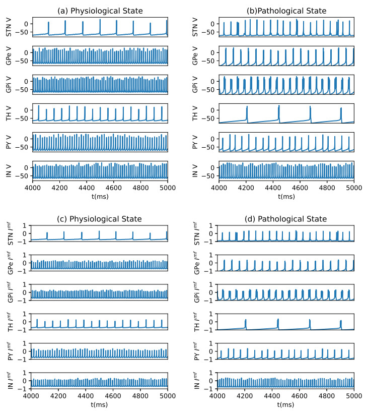
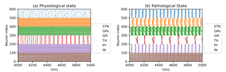
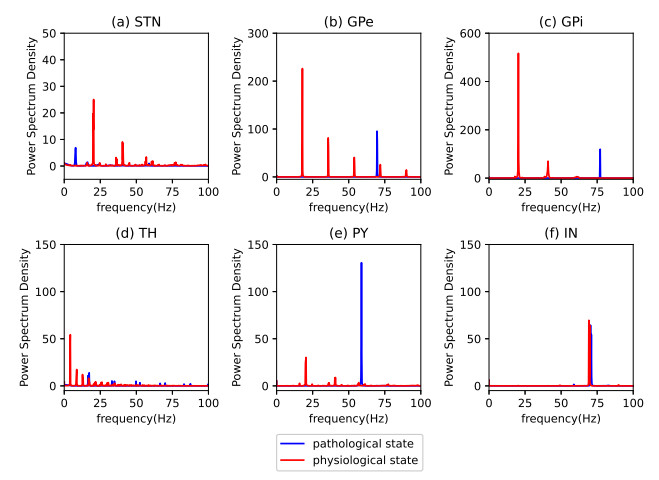
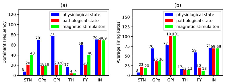
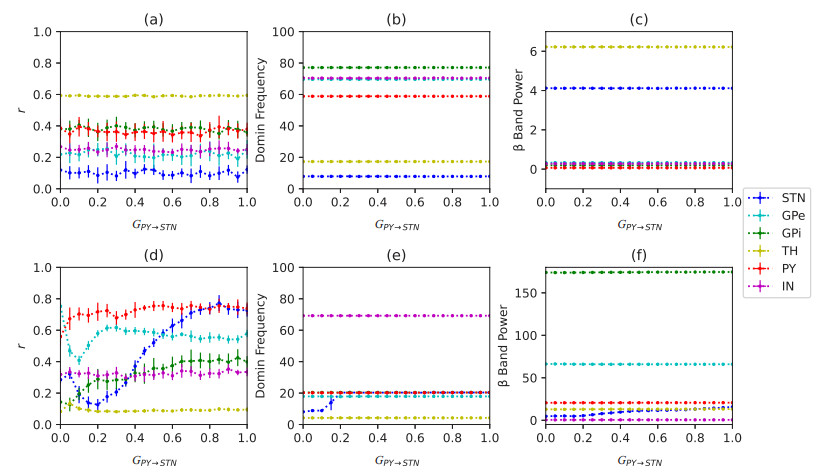
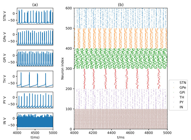
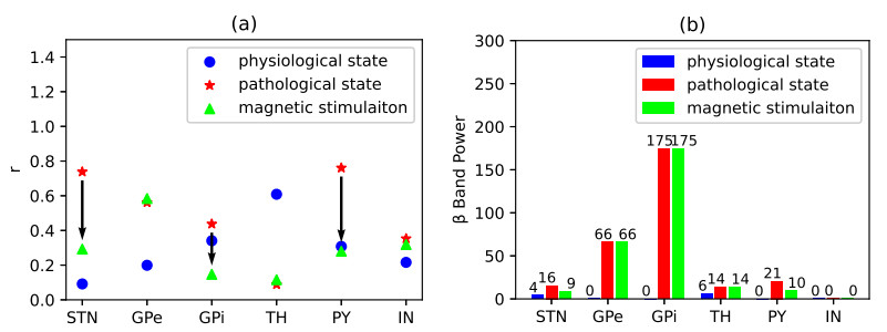
Parkinson's disease (PD) is mainly characterized by changes of firing and pathological oscillations in the basal ganglia (BG). In order to better understand the therapeutic effect of noninvasive magnetic stimulation, which has been used in the treatment of PD, we employ the Izhikevich neuron model as the basic node to study the electrical activity and the controllability of magnetic stimulation in a cortico-basal ganglia-thalamus (CBGT) network. Results show that the firing properties of the physiological and pathological state can be reproduced. Additionally, the electrical activity of pyramidal neurons and strong synapse connection in the hyperdirect pathway cause abnormal $\beta$ -band oscillations and excessive synchrony in the subthalamic nucleus (STN). Furthermore, the pathological firing properties of STN can be efficiently suppressed by external magnetic stimulation. The statistical results give the fitted boundary curves between controllable and uncontrollable regions. This work helps to understand the dynamic response of abnormal oscillation in the PD-related nucleus and provides insights into the mechanisms behind the therapeutic effect of magnetic stimulation.

Keywords:

Citation: Zilu Cao, Lin Du, Honghui Zhang, Lianghui Qu, Luyao Yan, Zichen Deng. Firing activities and magnetic stimulation effects in a Cortico-basal ganglia-thalamus neural network[J]. Electronic Research Archive, 2022, 30(6): 2054-2074. doi: 10.3934/era.2022104

Related Papers:

[1]	Yanyan Cui, Chaojun Wang . Dirichlet and Neumann boundary value problems for bi-polyanalytic functions on the bicylinder. AIMS Mathematics, 2025, 10(3): 4792-4818. doi: 10.3934/math.2025220
[2]	Yanyan Cui, Chaojun Wang . Systems of two-dimensional complex partial differential equations for bi-polyanalytic functions. AIMS Mathematics, 2024, 9(9): 25908-25933. doi: 10.3934/math.20241265
[3]	Kedong Wang, Xianguo Geng, Mingming Chen, Ruomeng Li . Long-time asymptotics for the generalized Sasa-Satsuma equation. AIMS Mathematics, 2020, 5(6): 7413-7437. doi: 10.3934/math.2020475
[4]	Iman Ben Othmane, Lamine Nisse, Thabet Abdeljawad . On Cauchy-type problems with weighted R-L fractional derivatives of a function with respect to another function and comparison theorems. AIMS Mathematics, 2024, 9(6): 14106-14129. doi: 10.3934/math.2024686
[5]	Jinfang Li, Chunjiang Wang, Li Zhang, Jian Zhang . Multi-solitons in the model of an inhomogeneous optical fiber. AIMS Mathematics, 2024, 9(12): 35645-35654. doi: 10.3934/math.20241691
[6]	Andrey Muravnik . Wiener Tauberian theorem and half-space problems for parabolic and elliptic equations. AIMS Mathematics, 2024, 9(4): 8174-8191. doi: 10.3934/math.2024397
[7]	Hassan Khan, Umar Farooq, Fairouz Tchier, Qasim Khan, Gurpreet Singh, Poom Kumam, Kanokwan Sitthithakerngkiet . The analytical analysis of fractional order Fokker-Planck equations. AIMS Mathematics, 2022, 7(7): 11919-11941. doi: 10.3934/math.2022665
[8]	Andrey Muravnik . Nonclassical dynamical behavior of solutions of partial differential-difference equations. AIMS Mathematics, 2025, 10(1): 1842-1858. doi: 10.3934/math.2025085
[9]	Naveed Iqbal, Azmat Ullah Khan Niazi, Ikram Ullah Khan, Rasool Shah, Thongchai Botmart . Cauchy problem for non-autonomous fractional evolution equations with nonlocal conditions of order $ (1, 2) $. AIMS Mathematics, 2022, 7(5): 8891-8913. doi: 10.3934/math.2022496
[10]	Meijiao Wang, Qiuhong Shi, Maoning Tang, Qingxin Meng . Stochastic differential equations in infinite dimensional Hilbert space and its optimal control problem with Lévy processes. AIMS Mathematics, 2022, 7(2): 2427-2455. doi: 10.3934/math.2022137

Abstract

1. Introduction

The Cauchy integral representations play an important role in the function theory of one or several complex variables, among which the Cauchy integral formula and the Cauchy-Pompeiu formula ^[1] are the two most important categories. The classical Cauchy-Pompeiu formulas ^[2] in $\mathbb{C}$ are:

$\begin{equation} \begin{aligned} w(z) = \frac{1}{2\pi i}\!\int_{\partial G}w(\zeta)\frac{d\zeta}{\zeta-z} -\frac{1}{\pi}\!\int_{G}w_{\bar{\zeta}}(\zeta)\frac{d\xi d\eta}{\zeta-z}, \quad z\in G, \end{aligned} \end{equation}$

(1.1)

$\begin{equation} \begin{aligned} w(z) = -\frac{1}{2\pi i}\!\int_{\partial G}w(\zeta)\frac{d\bar{\zeta}}{\overline{\zeta-z}} -\frac{1}{\pi}\!\int_{G}w_{\zeta}(\zeta)\frac{d\xi d\eta}{\overline{\zeta-z}}, \quad z\in G, \end{aligned} \end{equation}$

(1.2)

where $G$ is a bounded smooth domain in the complex plane and $w\in C^1(G; \mathbb{C})\bigcap C(\overline{G}; \mathbb{C})$ .

Obviously, the classical Cauchy-Pompeiu formulas are closely related to complex partial differential operators. Thus, lots of boundary value problems related to complex partial differential equations were solved with the help of the Cauchy integral formula and the Cauchy-Pompeiu formula in the complex plane $\mathbb{C}$ , see ^[3,4,5,6]. By iterating the Cauchy-Pompeiu formula for one variable, the solutions to second order systems in polydomains composed by the Laplace and the Bitsadze operators were obtained ^[7]. The Riemann-Hilbert problems for generalized analytic vectors and complex elliptic partial differential equations of higher order were investigated in $\mathbb{C}$ ^[8]. By constructing a weighted Cauchy-type kernel, the Cauchy-Pompeiu integral representation in the constant weights case and orthogonal case were obtained ^[9]. The classical Cauchy-Pompeiu formula was generalized to different cases for different kinds of functions in $\mathbb{C}$ ^[7], among which a high order case is:

$\begin{equation} w(z) = \sum\limits^{m-1}_{\mu = 0}\frac{1}{2\pi i}\!\int_{\partial G}\frac{1}{\mu!}\frac{(\overline{z-\zeta})^{\mu}}{\zeta-z}\partial^{\mu}_{\bar{\zeta}}w(\zeta)d\zeta -\frac{1}{\pi}\!\int_{G}\frac{1}{(m-1)!}\frac{(\overline{z-\zeta})^{m-1}}{\zeta-z}\partial^{m}_{\bar{\zeta}}w(\zeta)d\xi d\eta, \end{equation}$

(1.3)

where $w\in C^m(G; \mathbb{C})\bigcap C^{m-1}(\overline{G}; \mathbb{C})$ and $1\leq m$ , see ^[10]. The first item in the right hand of (1.3) is the Cauchy integral expression for $m$ -holomorphic functions on $D$ , and the second item in (1.3) is a singular integral operator. Let

$\begin{equation} T_{0, m}f(z) = \frac{-1}{\pi}\int_D\frac{1}{(m-1)!}\frac{(\overline{z-\zeta})^{m-1}}{\zeta-z}f(\zeta)d\xi d\eta, \end{equation}$

(1.4)

where $m\geq 1$ , $f\in C(\partial G)$ with $G$ being a bounded domain in the complex plane, then

$\begin{equation*} \frac{\partial^{m}T_{0, m}f(z)}{\partial \bar{z}^{m}} = f(z), \end{equation*}$

see ^[11]. Therefore, the solution to $\partial^m_{\bar{z}}w(z) = f(z)$ can be expressed as (1.3), and $T_{0, m}f(z)$ provides a particular solution to $\partial^m_{\bar{z}}w(z) = f(z)$ . Thus it can be seen that, the Cauchy-Pompeiu formulas provide the integral representations of solutions to some partial differential equations.

The generalizations of the classical Cauchy-Pompeiu formula have contributed to the flourishing development of boundary value problems in $\mathbb{C}$ . Many types of boundary value problems for analytic functions or polyanalytic functions have emerged in $\mathbb{C}$ . Among them, Riemann boundary value problems and Dirichlet problems are the two major categories. By using the Cauchy-Pompeiu formula and its generalizations, the solvable conditions were found, and the integral expressions of the solutions to some problems were obtained. Some were discussed on different ranges of the unit disk, such as a generalized Cauchy-Riemann equation with super-singular points on a half-plane ^[12], the variable exponent Riemann boundary value problem for Liapunov open curves ^[13], Schwarz boundary value problems for polyanalytic equation in a sector ring ^[14], and so on ^[15,16,17]. Some were investigated for different equations, such as bi-harmonic equations with a p-Laplacian ^[18] and so on ^[12,19,20], which are different from the partial differential equations in ^[7].

As we all know, analytic functions are defined by a pair of Cauchy-Riemann equations. Bi-analytic functions ^[21] arise from the generalized system of Cauchy-Riemann equations

$\begin{equation*} \left\{ \begin{array}{ll} \frac{\partial u}{\partial x}-\frac{\partial v}{\partial y} = \theta, \quad \frac{\partial u}{\partial y}+\frac{\partial v}{\partial x} = \omega, \\ (k+1)\frac{\partial \theta}{\partial x}+\frac{\partial \omega}{\partial y} = 0, \quad (k+1)\frac{\partial \theta}{\partial y}-\frac{\partial \omega}{\partial x} = 0, \end{array} \right. \end{equation*}$

where $k\in \mathbb{R}, \; k\neq -1$ , $\phi(z) = (k+1)\theta-i\omega$ is called the associated function of $f(z) = u+iv$ . A special case of bi-analytic functions is

$\begin{equation*} \partial_{\bar{z}}f(z) = \frac{\lambda-1}{4\lambda}\phi(z)+\frac{\lambda+1}{4\lambda}\overline{\phi(z)}, \quad \partial_{\bar{z}}\phi(z) = 0. \end{equation*}$

Bi-analytic functions are generalizations of analytic functions. They are important to studying elasticity problems and, therefore, have attracted the attention of many scholars. Begehr and Kumar ^[22] successfully obtained the solution to the Schwarz and Neumann boundary value problems for bi-polyanalytic functions. Lin and Xu ^[23] investigated the Riemann problem for ( $\lambda, k$ ) bi-analytic functions. There are many other excellent conclusions as well ^[24,25].

So far, there have been few results for boundary value problems of bi-analytic functions with Riemann-Hilbert boundary conditions. Stimulated by this, we investigate this type of problems for bi-polyanalytic functions ^[26]

$\begin{equation*} \partial_{\bar{z}}f(z) = \frac{\lambda-1}{4\lambda}\phi(z)+\frac{\lambda+1}{4\lambda}\overline{\phi(z)}, \quad \partial^n_{\bar{z}}\phi(z) = 0\; \; (n\geq 1), \end{equation*}$

where $\lambda\in\mathbb{R}\backslash\{-1, 0, 1\}$ , which are the extensions of bi-analytic functions.

To solve the boundary value problems for bi-polyanalytic functions, in this paper, we first discuss a Riemann-Hilbert problem related to complex partial differential operators of higher order on the unit disk, and then we investigate the boundary value problems for bi-polyanalytic functions with the Dirichlet and Riemann-Hilbert boundary conditions, the half-Neumann boundary conditions and the mixed boundary conditions. Applying this method, we can also discuss other related systems of complex partial differential equations of higher order for bi-polyanalytic functions.

2. Some lemmas

Let $\Re{z}$ and $\Im{z}$ represent the real and imaginary parts of the complex number $z$ , respectively. Let $C^m(G)$ represent the set of functions whose partial derivatives of order $m$ are all continuous within $G$ , and $C(G)$ represent the set of continuous functions on $G$ . To get the main results, we need the following lemmas:

Lemma 2.1. ^[2] Let $G$ be a bounded smooth domain in the complex plane, $f\in L_1(G; \mathbb{C})$ and

$\begin{equation*} Tf(z) = \frac{-1}{\pi}\int_G\frac{f(\zeta)}{\zeta-z}d\xi d\eta, \end{equation*}$

then $\partial_{\bar{z}}Tf(z) = f(z)$ .

Lemma 2.2. Let $D$ be the unit disk in $\mathbb{C}$ . For $\varphi\in C(\partial D, \mathbb{R})$ and $f_1\in C^{m-1}(\bar{D}, \mathbb{C})$ ( $m\geq 1$ ) with $\partial_{\bar{z}}f_{\kappa-1} = f_{\kappa}\; (\kappa = 2, \cdots\!, m), f_m = 0$ , let

$\begin{equation} \begin{aligned} \quad\quad\quad\quad\quad\quad\quad W(z)& = \frac{1}{2\pi i}\!\int_{\partial D}\varphi(\zeta)\frac{\zeta+z}{\zeta-z}\frac{d\zeta}{\zeta}+\frac{1}{2\pi i}\int_{\partial D}\sum\limits^{m-1}_{\mu = 1}\frac{1}{\mu!}\Re[(\overline{z-\zeta})^{\mu}f_{\mu}(\zeta)]\frac{\zeta+z}{\zeta-z}\frac{d\zeta}{\zeta}\\ &\quad+\frac{1}{2\pi}\int_{\partial D}\sum\limits^{m-1}_{\mu = 0}\frac{1}{\mu!}\Im\{[(\overline{z\!-\!\zeta})^{\mu}-(-\bar{\zeta}^{\mu})]f_{\mu}(\zeta)\} \frac{d\zeta}{\zeta}, \end{aligned} \end{equation}$

(2.1)

then $\Re W = \varphi$ , $\partial_{\bar{z}}^mW(z) = 0$ and $\partial_{\bar{z}}^sW(z) = f_s(z)\; (s = 1, 2, \cdots\!, m-1)$ .

Proof. $\Re W = \varphi$ is due to the property of the Schwarz operator, as $\frac{\zeta+z}{\zeta-z}$ is a pure imaginary number if $z\rightarrow \partial D$ .

Let

$\begin{equation*} \left\{ \begin{array}{cccc} A = \frac{1}{2\pi i}\!\int_{\partial D}\sum\limits^{m-1}_{\mu = 1}\!\frac{1}{\mu!}\Re[(\overline{z-\zeta})^{\mu}f_{\mu}(\zeta)]\frac{\zeta+z}{\zeta-z}\frac{d\zeta}{\zeta}, \\ B = \frac{1}{2\pi}\!\int_{\partial D}\sum\limits^{m-\!1}_{\mu = 0}\!\frac{1}{\mu!}\Im\{[(\overline{z\!-\!\zeta})^{\mu}\!-\!\!(-\bar{\zeta}^{\mu})]f_{\mu}(\zeta)\} \frac{d\zeta}{\zeta}. \end{array} \right. \end{equation*}$

Then

$\begin{equation} \left\{ \begin{array}{ll} \!\!A_{\bar{z}} = \! \sum\limits^{m-1}_{\mu = 1}\!\frac{1}{\mu!}\Big[\frac{1}{2\pi i}\int_{\partial D}\mu(\overline{z\!-\!\zeta})^{\mu-1}f_{\mu}(\zeta)\frac{d\zeta}{\zeta\!-\!z} \!-\!\frac{1}{2\pi i}\!\int_{\partial D}\mu(\overline{z\!-\!\zeta})^{\mu-1}f_{\mu}(\zeta)\frac{d\zeta}{2\zeta}\Big], \\ \!\!A_{\bar{z}}^s = \! \sum\limits^{m-1}_{\mu = s}\!\frac{1}{(\mu\!-\!s)!}\!\Big[\!\frac{1}{2\pi i}\!\!\int_{\!\partial D}\!\!(\overline{z\!-\!\zeta})^{\mu-s}\frac{f_{\mu}d\zeta}{\zeta\!-\!z} \!-\!\frac{1}{2\pi i}\!\int_{\!\partial D}\!\!(\overline{z\!-\!\zeta})^{\mu-s}\frac{f_{\mu}d\zeta}{2\zeta}\Big]\; (s = 2, \cdots\!, m\!-\!1), \\ \!\!A_{\bar{z}}^m = 0, \end{array} \right. \end{equation}$

(2.2)

and

$\begin{equation} \left\{ \begin{array}{ll} \!\!B_{\bar{z}} = \! \sum\limits^{m-\!1}_{\mu = 1}\!\!\frac{1}{4\pi i\mu!}\!\int_{\partial D}\mu(\overline{z\!-\!\zeta})^{\mu-1}f_{\mu}(\zeta)\frac{d\zeta}{\zeta}, \\ \!\!B_{\bar{z}}^s = \! \sum\limits^{m-\!1}_{\mu = s}\!\!\frac{1}{4\pi i(\mu-s)!}\!\int_{\partial D}(\overline{z\!-\!\zeta})^{\mu-s}f_{\mu}(\zeta)\frac{d\zeta}{\zeta}\; \; (s = 2, \cdots\!, m\!-\!1), \\ \!\!B_{\bar{z}}^m = 0. \end{array} \right. \end{equation}$

(2.3)

By (2.2), (2.3), and the Cauchy-Pompeiu formula (1.1), we get

$\begin{equation*} \begin{aligned} W_{\bar{z}}& = A_{\bar{z}}+B_{\bar{z}} = \sum\limits^{m-1}_{\mu = 1}\frac{1}{\mu!}\frac{1}{2\pi i}\int_{\partial D}\mu(\overline{z\!-\!\zeta})^{\mu-1}f_{\mu}(\zeta)\frac{d\zeta}{\zeta\!-\!z} \\ & = \!\frac{1}{2\pi i}\!\!\int_{\partial D}\!\Big[\sum\limits^{m-1}_{\mu = 1}\frac{1}{(\mu\!-\!1)!}(\overline{z\!-\!\zeta})^{\mu-1}f_{\mu}(\zeta)\Big]\frac{d\zeta}{\zeta\!-\!z} \!+\!\frac{-1}{\pi}\int_{D}\frac{\partial}{\partial\bar{\zeta}}\Big[\sum\limits^{m-1}_{\mu = 1}\frac{1}{(\mu\!-\!1)!}(\overline{z\!-\!\zeta})^{\mu-1}f_{\mu}(\zeta)\Big] \frac{d\sigma_{\zeta}}{\zeta-z}\\ & = \Big[\sum\limits^{m-1}_{\mu = 1}\!\!\frac{1}{(\mu\!-\!1)!}(\overline{z\!-\!\zeta})^{\mu-1}f_{\mu}(\zeta)\Big]_{\zeta = z} = f_1(z). \end{aligned} \end{equation*}$

Similarly,

$\begin{equation*} \partial_{\bar{z}}^sW(z) = \partial_{\bar{z}}^sA+\partial_{\bar{z}}^sB = f_s(z)\; \; (s = 2, \cdots\!, m-1), \; \; \partial_{\bar{z}}^mW(z) = \partial_{\bar{z}}^mA+\partial_{\bar{z}}^mB = 0. \end{equation*}$

□

Lemma 2.3. ^[11] Let $G$ be a bounded smooth domain in the complex plane, and $w\in$ $C^1(G; \mathbb{C})\bigcap C(\overline{G}; \mathbb{C})$ , then

$\begin{equation*} \int_{G}w_{\bar{z}}(z)dxdy = \frac{1}{2i}\int_{\partial G}w(z)dz, \int_{G}w_z(z)dxdy = -\frac{1}{2i}\int_{\partial G}w(z)d\bar{z}. \end{equation*}$

3. PDE of higher order with Riemann-Hilbert condition

Theorem 3.1. Let $D$ be the unit disk in $\mathbb{C}$ . For $\gamma, f_k\in C(\partial D)$ with $\partial_{\bar{z}}f_{k} = f_{k+1}$ ( $\; k\geq 1, k\in \mathbb{Z}$ ), let

$\begin{equation} T_{0, k}f_k(z) = \frac{-1}{\pi}\int_D\frac{1}{(k-1)!}\frac{(\overline{z-\zeta})^{k-1}}{\zeta-z}f_k(\zeta)d\sigma_{\zeta}, \end{equation}$

(3.1)

then the problem

$\begin{equation*} \left\{ \begin{array}{ll} \Re[\overline{\zeta}^pW(\zeta)] = \gamma(\zeta) \quad(\zeta\in\partial D), \\ \frac{\partial^{k}W(z)}{\partial \bar{z}^{k}} = f_{k}(z) \quad(z\in D) \end{array} \right. \end{equation*}$

is solvable on $D$ .

(i) In the case of $p\geq 0$ , the solution can be expressed as:

$\begin{equation} W(z) = z^p\varphi_1(z)+ \sum\limits^{k-1}_{s = 0}\sum\limits^s_{l = 0}\sum\limits^{+\infty}_{v = 0}\alpha_{sl(v-p)}z^v\bar{z}^l+T_{0, k}f_k(z), \end{equation}$

(3.2)

where

$\begin{equation} \begin{aligned} \varphi_1(z)& = \frac{1}{2\pi i}\int_{\partial D}\gamma(\zeta)\frac{\zeta+z}{\zeta-z}\frac{d\zeta}{\zeta} -\!\frac{1}{(k\!-\!1)!}\frac{z^{p}}{\pi}\!\!\int_D\!\!\overline{f_k(\zeta)}\frac{z(z-\zeta)^{k-1}}{1-z\bar{\zeta}}d\sigma_{\zeta}\\ &\quad+\frac{1}{2\pi i}\int_{\partial D}\sum\limits_{\mu = 1}^{k-1}\frac{1}{\mu!}\Re\Big[\overline{(z-\zeta)}^{\mu} \sum\limits^{\mu}_{m = 0}C^m_{\mu}(f_{\mu-m}(\zeta)-T_{0, k-\mu+m}f_k(\zeta))\partial^{m}_{\bar{\zeta}}\bar{\zeta}^p\Big]\frac{\zeta+z}{\zeta-z} \frac{d\zeta}{\zeta}\\ &\quad+\!\frac{1}{2\pi}\!\!\int_{\!\partial D}\!\sum\limits_{\mu = 0}^{k-1}\!\frac{1}{\mu!}\Im\Big[(\overline{(z\!-\!\zeta)}^{\mu}\!-\!\overline{(-\zeta)}^{\mu}) \!\!\sum\limits^{\mu}_{m = 0}\!\!C^m_{\mu}(f_{\mu-m}(\zeta)\!-\!T_{0, k-\mu+m}f_k(\zeta))\partial^{m}_{\bar{\zeta}}\bar{\zeta}^p\Big] \frac{d\zeta}{\zeta}, \end{aligned} \end{equation}$

(3.3)

$\alpha_{sl(v-p)}$ are arbitrary complex constants satisfying

$\begin{equation} \left\{ \begin{array}{ll} \sum\limits^{k-1}_{s = 0}\sum\limits^{s}_{l = 0}\!\alpha_{sl(v+l)} = 0 \; (v\!\geq\! p\!+\!k), \; \sum\limits^{k-1}_{s = 0}\sum\limits^{s}_{l = 0}[\alpha_{sl(v+l)}+\overline{\alpha_{sl(l-v)}}] = 0 \; (-p\!\leq\! v\!\leq\! p), \\ \sum\limits^{k-1}_{s = 0}\!\sum\limits^{s}_{l = 0}\!\alpha_{sl(p+1+t+l)}\! +\!\!\sum\limits^{k-1}_{s = t+1}\sum\limits^{s}_{l = t+1}\!\overline{\alpha_{sl(-p-1-t+l)}} = 0 \; \; (t = 0, 1, \cdots, k-2, \; k\geq2). \end{array} \right. \end{equation}$

(3.4)

For $k = 1$ the last equation in (3.4) is non-existent.

(ii) In the case of $p < 0$ , the solution can be expressed as:

$\begin{equation} W(z) = z^p\varphi_2(z)+ \sum\limits^{k-1}_{s = 0}\sum\limits^s_{l = 0}\sum\limits^{+\infty}_{v = 0}\alpha_{sl(v-p)}z^v\bar{z}^l+T_{0, k}f_k(z) \end{equation}$

(3.5)

on the condition that

$\begin{equation} \!\frac{1}{2\pi i}\!\!\int_{\partial D}\!\!\!\{\zeta^{-p}[f_{k-1}(\zeta)\!-\!T_{0, 1}f_k(\zeta)]+\zeta^{p}[\overline{f_{k-1}(\zeta)\!-\!T_{0, 1}f_k(\zeta)}]\} \frac{d\zeta}{\zeta^{l+1}} = 0\; \; (l = 0, 1, \cdots\!, \!-\!p\!-\!1), \end{equation}$

(3.6)

where $\alpha_{sl(v-p)}$ is the same as in (i) and

$\begin{equation} \begin{aligned} \varphi_2(z)& = \frac{1}{2\pi i}\int_{\partial D}\gamma\frac{\zeta+z}{\zeta-z}\frac{d\zeta}{\zeta} -\!\frac{1}{(k\!-\!1)!}\frac{z^{p}}{\pi}\!\!\int_D\!\!\overline{f_k(\zeta)}\frac{z(z-\zeta)^{k-1}}{1-z\bar{\zeta}}d\sigma_{\zeta}\\ &\quad+\frac{1}{2\pi i}\int_{\partial D}\sum\limits_{\mu = 1}^{k-1}\frac{1}{\mu!}\Re\{\overline{(z-\zeta)}^{\mu}\zeta^{-p}[f_{\mu}(\zeta)-T_{0, (k-\mu)}f_k(\zeta)]\}\frac{\zeta+z}{\zeta-z} \frac{d\zeta}{\zeta}\\ &\quad+\frac{1}{2\pi}\int_{\partial D}\sum\limits_{\mu = 0}^{k-1}\frac{1}{\mu!}\Im\{(\overline{(z-\zeta)}^{\mu}-\overline{(-\zeta)}^{\mu})\zeta^{-p}[f_{\mu}(\zeta)-T_{0, (k-\mu)}f_k(\zeta)]\} \frac{d\zeta}{\zeta}. \end{aligned} \end{equation}$

(3.7)

Proof. (1) For $n = 1$ , by Lemma 2.1, $T_{0, k}f_k(z)$ is a particular solution to $\frac{\partial^{k}W(z)}{\partial \bar{z}^{k}} = f_{k}(z)$ , then the corresponding general solution is $W(z) = \varphi(z)+T_{0, k}f_k(z)$ , where $\varphi(z)$ is a $k$ -holomorphic function with

$\begin{equation*} \Re[\zeta^{-p}\varphi(\zeta)] = \Re[\zeta^{-p}W(\zeta)-\zeta^{-p}T_{0, k}f_k(\zeta)] = \gamma(\zeta)-\Re[\zeta^{-p}T_{0, k}f_k(\zeta)]\doteq \gamma_0(\zeta). \end{equation*}$

(i) In the case of $p\geq 0 (p\in\mathbb{Z})$ :

① Let $\varphi(z) = z^p\varphi_1(z)$ , then $\Re[\zeta^{-p}\varphi(\zeta)] = \gamma_0(\zeta)\Leftrightarrow\Re[\varphi_1(\zeta)] = \gamma_0(\zeta)$ , and $\varphi(z)$ is $k$ -holomorphic if $\varphi_1(z)$ is $k$ -holomorphic. As

$\begin{equation*} \begin{aligned} \partial^{\mu}_{\bar{\zeta}}(\bar{\zeta}^p\varphi(\zeta))& = \sum\limits_{m = 0}^{\mu}C^m_{\mu}\partial^{\mu-m}_{\bar{\zeta}}\varphi(\zeta)\partial^{m}_{\bar{\zeta}}(\bar{\zeta}^p) = \sum\limits_{m = 0}^{\mu}C^m_{\mu}\partial^{\mu-m}_{\bar{\zeta}}[W(\zeta)-T_{0, k}f_k(\zeta)]\partial^{m}_{\bar{\zeta}}(\bar{\zeta}^p)\\ & = \sum\limits_{m = 0}^{\mu}C^m_{\mu}[f_{\mu-m}(\zeta)-T_{0, k-\mu+m}f_k(\zeta)]\partial^{m}_{\bar{\zeta}}(\bar{\zeta}^p), \end{aligned} \end{equation*}$

by Lemma 2.2 we get that

$\begin{equation} \begin{aligned} \varphi_1(z)& = \frac{1}{2\pi i}\int_{\partial D}\sum\limits_{\mu = 0}^{k-1}\frac{1}{\mu!}\Re[\overline{(z-\zeta)}^{\mu}\partial^{\mu}_{\bar{\zeta}}(\bar{\zeta}^p\varphi(\zeta))]\frac{\zeta+z}{\zeta-z} \frac{d\zeta}{\zeta}\\ &\quad+\frac{1}{2\pi}\int_{\partial D}\sum\limits_{\mu = 0}^{k-1}\frac{1}{\mu!}\Im[(\overline{(z-\zeta)}^{\mu}-\overline{(-\zeta)}^{\mu})\partial^{\mu}_{\bar{\zeta}}(\bar{\zeta}^p\varphi(\zeta))] \frac{d\zeta}{\zeta}\\ & = \frac{1}{2\pi i}\int_{\partial D}\gamma(\zeta)\frac{\zeta+z}{\zeta-z}\frac{d\zeta}{\zeta} -\frac{1}{2\pi i}\int_{\partial D}[\zeta^{-p}T_{0, k}f_k(\zeta)+\zeta^{p}\overline{T_{0, k}f_k(\zeta)}](\frac{1}{\zeta-z}-\frac{1}{2\zeta})d\zeta\\ &\quad+\frac{1}{2\pi i}\int_{\partial D}\sum\limits_{\mu = 1}^{k-1}\frac{1}{\mu!}\Re[\overline{(z-\zeta)}^{\mu} \sum\limits^{\mu}_{m = 0}C^m_{\mu}(f_{\mu-m}(\zeta)-T_{0, k-\mu+m}f_k(\zeta))\partial^{m}_{\bar{\zeta}}\bar{\zeta}^p]\frac{\zeta+z}{\zeta-z} \frac{d\zeta}{\zeta}\\ &\quad+\!\frac{1}{2\pi}\!\!\int_{\partial D}\!\sum\limits_{\mu = 0}^{k-1}\!\frac{1}{\mu!}\Im\Big[(\overline{(z\!-\!\zeta)}^{\mu}\!-\!\overline{(-\zeta)}^{\mu}) \!\!\sum\limits^{\mu}_{m = 0}\!\!C^m_{\mu}(f_{\mu-m}(\zeta)\!-\!T_{0, k-\mu+m}f_k(\zeta))\partial^{m}_{\bar{\zeta}}\bar{\zeta}^p\Big] \frac{d\zeta}{\zeta} \end{aligned} \end{equation}$

(3.8)

satisfies $\Re[\varphi_1(\zeta)] = \gamma_0(\zeta)$ and $\partial_{\bar{z}}^k\varphi_1(z) = 0$ . Furthermore, by (3.1), we obtain that

$\begin{equation} \begin{aligned} \frac{1}{2\pi i}\!\!\int_{\partial D}\!\!\!\zeta^{-p}T_{0, k}f_k(\zeta)\frac{d\zeta}{\zeta-z} & = \!\!\frac{1}{(k\!-\!1)!}\frac{-1}{\pi}\!\!\int_D\!\!f_k(\zeta')\Big[\frac{1}{2\pi i}\!\int_{\partial D}\!\!\zeta^{-p}\frac{(\overline{\zeta-\zeta'})^{k-1}}{\zeta'-\zeta}\frac{d\zeta}{\zeta-z}\Big]d\sigma_{\zeta'}\\ & = \!\!\frac{1}{(k\!-\!1)!}\frac{-1}{\pi}\!\!\int_D\!\!f_k(\zeta')\Big[\frac{-1}{2\pi i}\!\int_{\partial D}\!\!\bar{\zeta}^{p}\frac{(\overline{\zeta-\zeta'})^{k-1}}{\bar{\zeta}\zeta'-1}\frac{d\bar{\zeta}}{z\bar{\zeta}-1}\Big]d\sigma_{\zeta'} = \!0, \end{aligned} \end{equation}$

(3.9)

which follows

$\begin{equation} \frac{1}{2\pi i}\int_{\partial D}\zeta^{-p}T_{0, k}f_k(\zeta)\frac{d\zeta}{2\zeta} = 0. \end{equation}$

(3.10)

Meanwhile,

$\begin{equation} \begin{aligned} \frac{1}{2\pi i}\!\!\int_{\partial D}\!\!\!\zeta^{p}\overline{T_{0, k}f_k(\zeta)}\frac{d\zeta}{\zeta-z} & = \frac{1}{(k\!-\!1)!}\frac{-1}{\pi}\!\!\int_D\!\!\overline{f_k(\zeta')}\Big[\frac{1}{2\pi i}\!\int_{\partial D}\!\!\zeta^{p}\frac{(\zeta-\zeta')^{k-1}}{\bar{\zeta'}-\bar{\zeta}}\frac{d\zeta}{\zeta-z}\Big]d\sigma_{\zeta'}\\ & = \frac{1}{(k\!-\!1)!}\frac{-1}{\pi}\int_D\overline{f_k(\zeta')}\frac{z^{p+1}(z-\zeta')^{k-1}}{z\bar{\zeta'}-1}d\sigma_{\zeta'}\\ & = \frac{z^p}{(k\!-\!1)!}\frac{-1}{\pi}\int_D\overline{f_k(\zeta)}\frac{z(z-\zeta)^{k-1}}{z\bar{\zeta}-1}d\sigma_{\zeta}, \end{aligned} \end{equation}$

(3.11)

which follows

$\begin{equation} \frac{1}{2\pi i}\int_{\partial D}\zeta^{p}\overline{T_{0, k}f_k(\zeta)}\frac{d\zeta}{2\zeta} = 0. \end{equation}$

(3.12)

Plugging (3.9)–(3.12) into (3.8), we get (3.3). Therefore $z^p\varphi_1(z)$ is a particular solution to $\Re[\zeta^{-p}\varphi(\zeta)] = \gamma_0(\zeta)$ and $\partial_{\bar{z}}^k\varphi(z) = 0$ .

② If $\varphi_0(z)$ is $k$ -holomorphic on $D$ with $\Re[\zeta^{-p}\varphi_0(z)] = 0$ , then $z^p\varphi_1(z)+\varphi_0(\zeta)$ is the general solution to $\Re[\zeta^{-p}\varphi(\zeta)] = \gamma_0(\zeta)$ and $\partial_{\bar{z}}^k\varphi(z) = 0$ . In the following, we seek $\varphi_0(z)$ .

As $\varphi_0(z)$ is $k$ -holomorphic, it can be expressed as

$\begin{equation} \varphi_0(z) = \sum\limits^{k-1}_{s = 0}\sum\limits^s_{l = 0}\sum\limits^{+\infty}_{v = 0}C_{slv}z^v\bar{z}^l \doteq\sum\limits^{k-1}_{s = 0}\sum\limits^s_{l = 0}\sum\limits^{+\infty}_{v = 0}\alpha_{sl(v-p)}z^v\bar{z}^l, \end{equation}$

(3.13)

where $\alpha_{sl(v-p)} = C_{slv}$ are arbitrary complex constants. Let

$\begin{equation} \alpha_{slv}\!+\!\overline{\alpha_{sl(2l-v)}} = A_{slv}, \quad \alpha_{slv} = B_{slv}, \quad \overline{\alpha_{sl(2l-v)}} = C_{slv}, \end{equation}$

(3.14)

then

$\begin{equation} \begin{aligned} 0& = \Re\{\bar{\zeta}^p\varphi_0(\zeta)\} = \sum\limits^{k-1}_{s = 0}\sum\limits^s_{l = 0}\sum\limits^{+\infty}_{v = -p}(\alpha_{slv}\zeta^{v-l}+\overline{\alpha_{slv}}\zeta^{l-v})\\ & = \sum\limits^{k-1}_{s = 0}\sum\limits^s_{l = 0}\sum\limits^{p+2l}_{v = -p}(\alpha_{slv}+\overline{\alpha_{sl(2l-v)}})\zeta^{v-l} +\sum\limits^{k-1}_{s = 0}\sum\limits^s_{l = 0}\sum\limits^{+\infty}_{v = p+2l+1}\alpha_{slv}\zeta^{v-l} +\sum\limits^{k-1}_{s = 0}\sum\limits^s_{l = 0}\sum\limits^{-p-1}_{v = -\infty}\overline{\alpha_{sl(2l-v)}}\zeta^{v-l}\\ & = \sum\limits^{k-1}_{s = 0}\sum\limits^s_{l = 0}\sum\limits^{p+2l}_{v = -p}A_{slv}\zeta^{v-l} +\sum\limits^{k-1}_{s = 0}\sum\limits^s_{l = 0}\sum\limits^{+\infty}_{v = p+2l+1}B_{slv}\zeta^{v-l} +\sum\limits^{k-1}_{s = 0}\sum\limits^s_{l = 0}\sum\limits^{-p-1}_{v = -\infty}C_{slv}\zeta^{v-l}\\ & = \Big\{\sum\limits^{p}_{v = -p}\!\!\!A_{00v}\zeta^{v}+(\sum\limits^{p}_{v = -p}A_{10v}\zeta^{v}+\sum\limits^{p+2}_{v = -p}A_{11v}\zeta^{v-1}) +(\sum\limits^{p}_{v = -p}A_{20v}\zeta^{v}+\sum\limits^{p+2}_{v = -p}A_{21v}\zeta^{v-1}+\sum\limits^{p+4}_{v = -p}A_{22v}\zeta^{v-2})\\ &\quad+\cdots+\Big[\!\sum\limits^{p}_{v = -p}A_{(k-1)0v}\zeta^{v}\!+\!\!\sum\limits^{p+2}_{v = -p}A_{(k-1)1v}\zeta^{v-1}\! +\!\cdots\!+\!\!\sum\limits^{p+2(k-1)}_{v = -p}A_{(k-1)(k-1)v}\zeta^{v-(k-1)}\Big]\Big\}\\ &\quad+\Big\{\!\!\sum\limits^{+\infty}_{v = p+1}B_{00v}\zeta^{v}\!\!+\!\!(\!\sum\limits^{+\infty}_{v = p+1}B_{10v}\zeta^{v}\! \!+\!\!\!\!\sum\limits^{+\infty}_{v = p+3}B_{11v}\zeta^{v-1}\!) \!+\!(\!\sum\limits^{+\infty}_{v = p+1}B_{20v}\zeta^{v}\!\!+\!\!\!\sum\limits^{+\infty}_{v = p+3}B_{21v}\zeta^{v-1}\! \!+\!\!\!\sum\limits^{+\infty}_{v = p+5}B_{22v}\zeta^{v-2})\end{aligned} \end{equation}$

(3.15)

$\begin{equation} \begin{aligned} &\quad+\!\cdots\!+\Big[\!\sum\limits^{+\infty}_{v = p+1}\!\!\!B_{(k-1)0v}\zeta^{v}\!+\!\!\sum\limits^{+\infty}_{v = p+3}\!\!\!B_{(k-1)1v}\zeta^{v-1}\! +\!\cdots\!+\!\!\sum\limits^{+\infty}_{v = p+2k-1}\!\!\!B_{(k-1)(k-1)v}\zeta^{v-(k-1)}\Big]\Big\}\\ &\quad+\sum\limits^{-p-1}_{v = -\infty}\!\Big\{C_{00v}\zeta^{v}\!+\!(C_{10v}\zeta^{v}\! +C_{11v}\zeta^{v-1}\!) \!+\!(C_{20v}\zeta^{v}\!+\!C_{21v}\zeta^{v-1}\! +\!C_{22v}\zeta^{v-2})\\ &\quad+\!\cdots+\Big[C_{(k-1)0v}\zeta^{v}\!+\!C_{(k-1)1v}\zeta^{v-1}\! +\!\cdots\!+\!C_{(k-1)(k-1)v}\zeta^{v-(k-1)}\Big]\Big\}\\ & = \Big\{\sum\limits^{p}_{v = -p}\zeta^{v}\Big[\sum\limits^{k-1}_{l = 0}\sum\limits^{k-1}_{s = l}A_{sl(v+l)}\Big]+\zeta^{-p-1}\sum\limits^{k-1}_{l = 1}\sum\limits^{k-1}_{s = l}A_{sl(-p-1+l)} +\cdots+\zeta^{-p-k+1}A_{(k-1)(k-l)(-p)}\\ &\quad+\zeta^{p+1}\sum\limits^{k-1}_{l = 1}\sum\limits^{k-1}_{s = l}A_{sl(p+1+l)}+\zeta^{p+2}\sum\limits^{k-1}_{l = 2}\sum\limits^{k-1}_{s = l}A_{sl(p+2+l)} +\cdots+\zeta^{p+k-1}A_{(k-1)(k-1)(p+2(k-1))}\Big\}\\ &\quad+\Big\{\zeta^{p+1}\sum\limits^{k-1}_{s = 0}B_{s0(p+1)}+\zeta^{p+2}\Big[\sum\limits^{k-1}_{s = 0}B_{s0(p+2)}+\sum\limits^{k-1}_{s = 1}B_{s1(p+3)}\Big]\\ &\quad+\cdots+\zeta^{p+k-1}\sum\limits^{k-2}_{l = 0}\sum\limits^{k-1}_{s = l}B_{sl(p+k-1+l)} +\sum\limits^{+\infty}_{v = p+k}\zeta^v\Big[\sum\limits^{k-1}_{l = 0}\sum\limits^{k-1}_{s = l}B_{sl(v+l)}\Big]\Big\}\\ &\quad+\Big\{\zeta^{-p-1}\sum\limits^{k-1}_{s = 0}C_{s0(-p-1)}+\zeta^{-p-2}\Big[\sum\limits^{k-1}_{s = 0}C_{s0(-p-2)}+\sum\limits^{k-1}_{s = 1}C_{s1(-p-1)}\Big]\\ &\quad+\cdots+\zeta^{-p-k+1}\sum\limits^{k-2}_{l = 0}\sum\limits^{k-1}_{s = l}C_{sl(-p-k+1+l)} +\sum\limits^{-p-k}_{v = -\infty}\zeta^v\Big[\sum\limits^{k-1}_{l = 0}\sum\limits^{k-1}_{s = l}C_{sl(v+l)}\Big]\Big\}\\ & = \sum\limits^{-p-k}_{v = -\infty}\zeta^v\Big[\sum\limits^{k-1}_{l = 0}\sum\limits^{k-1}_{s = l}C_{sl(v+l)}\Big] +\zeta^{-p-k+1}\Big[\sum\limits^{k-2}_{l = 0}\sum\limits^{k-1}_{s = l}C_{sl(-p-k+1+l)}+A_{(k-1)(k-l)(-p)}\Big]+\cdots\\ &\quad+\zeta^{-p-1}\Big[\sum\limits^{k-1}_{s = 0}C_{s0(-p-1)}+\sum\limits^{k-1}_{l = 1}\sum\limits^{k-1}_{s = l}A_{sl(-p-1+l)}\Big] +\sum\limits^{p}_{v = -p}\zeta^{v}\Big[\sum\limits^{k-1}_{l = 0}\sum\limits^{k-1}_{s = l}A_{sl(v+l)}\Big]\\ &\quad+\!\zeta^{p+1}\Big[\sum\limits^{k-1}_{s = 0}\!B_{s0(p+1)}\!\!+\!\!\sum\limits^{k-1}_{l = 1}\sum\limits^{k-1}_{s = l}\!A_{sl(p+1+l)}\Big] +\zeta^{p+k-1}\Big[\sum\limits^{k-2}_{l = 0}\sum\limits^{k-1}_{s = l}\!B_{sl(p+k-1+l)}+A_{(k-1)(k-1)(p+2(k-1))}\Big]\\ &\quad+\sum\limits^{+\infty}_{v = p+k}\zeta^v\Big[\sum\limits^{k-1}_{l = 0}\sum\limits^{k-1}_{s = l}B_{sl(v+l)}\Big], \end{aligned} \end{equation}$

(3.16)

which leads to (3.4) in consideration of (3.14) and

$\begin{equation*} \sum\limits^{k-1}_{l = 0}\sum\limits^{k-1}_{s = l}C_{slv} = \sum\limits^{k-1}_{s = 0}\sum\limits^{s}_{l = 0}C_{slv}. \end{equation*}$

By ① and ②, (3.2) is the solution to Problem RH.

(ii) In the case of $p < 0 (p\in\mathbb{Z})$ :

① Let $\varphi(z) = z^p\varphi_2(z)$ , then $\Re[\zeta^{-p}\varphi(\zeta)] = \gamma_0(\zeta)\Leftrightarrow\Re[\varphi_2(\zeta)] = \gamma_0(\zeta)$ . Similar to the discussion of ① in (i), we get a particular solution $\varphi_2(z)$ for $\Re[\varphi_2(\zeta)] = \gamma_0(\zeta)$ where $\varphi_2(z)$ is $k$ holomorphic:

$\begin{equation*} \begin{aligned} \varphi_2(z)& = \frac{1}{2\pi i}\int_{\partial D}\gamma_0\frac{\zeta+z}{\zeta-z}\frac{d\zeta}{\zeta} +\frac{1}{2\pi i}\int_{\partial D}\sum\limits_{\mu = 1}^{k-1}\frac{1}{\mu!}\Re[\overline{(z-\zeta)}^{\mu}\zeta^{-p}\partial^{\mu}_{\bar{\zeta}}\varphi(\zeta)]\frac{\zeta+z}{\zeta-z} \frac{d\zeta}{\zeta}\\ &+\frac{1}{2\pi}\int_{\partial D}\sum\limits_{\mu = 0}^{k-1}\frac{1}{\mu!}\Im[(\overline{(z-\zeta)}^{\mu}-\overline{(-\zeta)}^{\mu})\zeta^{-p}\partial^{\mu}_{\bar{\zeta}}\varphi(\zeta)] \frac{d\zeta}{\zeta}\\ & = \frac{1}{2\pi i}\int_{\partial D}\gamma\frac{\zeta+z}{\zeta-z}\frac{d\zeta}{\zeta}-\frac{1}{2\pi i}\int_{\partial D}[\zeta^{-p}T_{0, k}f_k(\zeta)+\zeta^{p}\overline{T_{0, k}f_k(\zeta)}](\frac{1}{\zeta-z}-\frac{1}{2\zeta})d\zeta\\ &\quad+\frac{1}{2\pi i}\int_{\partial D}\sum\limits_{\mu = 1}^{k-1}\frac{1}{\mu!}\Re[\overline{(z-\zeta)}^{\mu}\zeta^{-p}\partial^{\mu}_{\bar{\zeta}}\varphi(\zeta)]\frac{\zeta+z}{\zeta-z} \frac{d\zeta}{\zeta}\\ &\quad+\frac{1}{2\pi}\int_{\partial D}\sum\limits_{\mu = 0}^{k-1}\frac{1}{\mu!}\Im[(\overline{(z-\zeta)}^{\mu}-\overline{(-\zeta)}^{\mu})\zeta^{-p}\partial^{\mu}_{\bar{\zeta}}\varphi(\zeta)] \frac{d\zeta}{\zeta}. \end{aligned} \end{equation*}$

So we get (3.7) for (3.9)–(3.12) and

$\begin{equation*} \partial^{\mu}_{\bar{\zeta}}\varphi(\zeta) = \partial^{\mu}_{\bar{\zeta}}[W(\zeta)-T_{0, k}f_k(\zeta)] = \partial^{\mu}_{\bar{\zeta}}W(\zeta)-\partial^{\mu}_{\bar{\zeta}}T_{0, k}f_k(\zeta) = f_{\mu}(\zeta)-T_{0, (k-\mu)}f_k(\zeta). \end{equation*}$

Therefore

$\begin{equation*} \varphi(z) = z^p\varphi_2(z)+\sum\limits^{k-1}_{s = 0}\sum\limits^s_{l = 0}\sum\limits^{+\infty}_{v = 0}\alpha_{sl(v-p)}z^v\bar{z}^l \end{equation*}$

is the solution to $\Re[\zeta^{-p}\varphi(\zeta)] = \gamma_0(\zeta)$ and $\partial_{\bar{z}}^k\varphi(z) = 0$ , where $\alpha_{sl(v-p)}$ are arbitrary complex constants satisfying (3.12).

② Secondly, we seek the condition to ensure that $\varphi(z)$ is $k$ -holomorphic from $\varphi_2(z) = z^{-p}\varphi(z)$ . As the $k$ -holomorphism of $\varphi_2(z) = z^{-p}\varphi(z)$ is equivalent to the holomorphism of $\partial_{\bar{z}}^{k-1}\varphi_2(z) = z^{-p}\partial_{\bar{z}}^{k-1}\varphi(z)$ , applying the properties of the Schwarz operator for holomorphic functions and

$\begin{equation*} \frac{1}{\zeta-z} = \frac{1}{\zeta}\cdot\frac{1}{1-\frac{z}{\zeta}} = \sum\limits^{\infty}_{l = 0}\frac{z^l}{\zeta^{l+1}}\quad (|\frac{z}{\zeta}| < 1), \end{equation*}$

we get that

$\begin{equation*} \begin{aligned} z^{-p}\partial_{\bar{z}}^{k-1}\varphi(z)& = \frac{1}{2\pi i}\int_{\partial D}[\zeta^{-p}\partial_{\bar{\zeta}}^{k-1}\varphi(\zeta)+\zeta^{p}\overline{\partial_{\bar{\zeta}}^{k-1}\varphi(\zeta)}] \Big[\frac{2\zeta}{\zeta-z}-1\Big]\frac{d\zeta}{2\zeta}\\ & = \sum\limits^{\infty}_{l = 0}\Big\{\frac{1}{2\pi i}\int_{\partial D}[\zeta^{-p}\partial_{\bar{\zeta}}^{k-1}\varphi(\zeta)+\zeta^{p}\overline{\partial_{\bar{\zeta}}^{k-1}\varphi(\zeta)}] \frac{d\zeta}{\zeta^{l+1}}\Big\}z^l\\ &\quad-\frac{1}{2\pi i}\int_{\partial D}[\zeta^{-p}\partial_{\bar{\zeta}}^{k-1}\varphi(\zeta)+\zeta^{p}\overline{\partial_{\bar{\zeta}}^{k-1}\varphi(\zeta)}] \frac{d\zeta}{2\zeta}. \end{aligned} \end{equation*}$

As $p < 0$ , then $\varphi(z)$ is $k$ -holomorphic (-i.e., $\partial_{\bar{z}}^{k-1}\varphi(z)$ is holomorphic) if and only if $z^{-p}\partial_{\bar{z}}^{k-1}\varphi(z)$ has a zero of order at least $-p$ at $z = 0$ . Therefore,

$\begin{equation*} \frac{1}{2\pi i}\int_{\partial D}[\zeta^{-p}\partial_{\bar{\zeta}}^{k-1}\varphi(\zeta)+\zeta^{p}\overline{\partial_{\bar{\zeta}}^{k-1}\varphi(\zeta)}] \frac{d\zeta}{\zeta^{l+1}} = 0\; \; (l = 0, 1, \cdots, -p-1), \end{equation*}$

that is (3.6) as

$\begin{equation*} \partial^{k-1}_{\bar{\zeta}}\varphi(\zeta) = \partial^{k-1}_{\bar{\zeta}}[W(\zeta)-T_{0, k}f_k(\zeta)] = \partial^{k-1}_{\bar{\zeta}}W(\zeta)-\partial^{k-1}_{\bar{\zeta}}T_{0, k}f_k(\zeta) = f_{k-1}(\zeta)-T_{0, 1}f_k(\zeta). \end{equation*}$

By ① and ②, (3.5) is the solution of Problem RH on the condition of (3.6).

Theorem 3.1 extends the conclusions of Riemann-Hilbert boundary value problems for k-holomorphic functions. Given that $k = 1$ in Theorem 3.1, we can get the following conclusion, which extends the existing results of the corresponding Riemann-Hilbert problems for analytic functions. □

Corollary 3.2. Let $D$ be the unit disk in $\mathbb{C}$ . For $\gamma, f\in C(\partial D)$ , the problem

$\begin{equation*} \Re[\bar{\zeta}^pW(\zeta)] = \gamma(\zeta) \; (\zeta\in\partial D), \quad \frac{\partial W(z)}{\partial \bar{z}} = f(z) \; (z\in D) \end{equation*}$

is solvable on $D$ .

(i) In the case of $p\geq 0$ , the solution can be expressed as:

$\begin{equation*} W(z) = \frac{z^p}{2\pi i}\int_{\partial D}\gamma(\zeta)\frac{\zeta+z}{\zeta-z}\frac{d\zeta}{\zeta} -\frac{z^{2p+1}}{\pi}\int_D\frac{\overline{f(\zeta)}}{1-z\bar{\zeta}}d\sigma_{\zeta} + \sum\limits^{2p}_{v = 0}\alpha_{v-p}z^v-\frac{1}{\pi}\int_D\frac{f(\zeta)}{\zeta-z}d\sigma_{\zeta}, \end{equation*}$

where $\alpha_{v-p}$ are arbitrary complex constants satisfying $\alpha_v+\overline{\alpha_{-v}} = 0 \; (-p\!\leq\! v\!\leq\! p)$ ;

(ii) In the case of $p < 0$ , the solution is the same as in (i) on the condition of

$\begin{equation*} \frac{1}{2\pi i}\int_{\partial D}\{\gamma(\zeta)-\Re[\zeta^{-p}Tf(\zeta)]\} \frac{d\zeta}{\zeta^{l+1}} = 0\; \; (l = 0, 1, \cdots, -p-1). \end{equation*}$

4. PDE for bi-polyanalytic functions

In this section we discuss several boundary value problems for bi-polyanalytic functions with the Dirichlet, Riemann-Hilbert boundary conditions or the mixed boundary conditions.

Theorem 4.1. Let $D$ be the unit disk in $\mathbb{C}$ , and let $\lambda\in\mathbb{R}\backslash\{-1, 0, 1\}$ , $\varphi, \gamma, f_k\in C(\partial D)$ with $\partial_{\bar{z}}f_{k} = f_{k+1}$ ( $\; k = 1, 2, \cdots, n-1, \; n\geq 2$ ) and $f_n = 0$ . Then the problem

$\begin{equation} \left\{ \begin{array}{ll} \partial_{\bar{z}}f(z) = \frac{\lambda-1}{4\lambda}\phi(z)+\frac{\lambda+1}{4\lambda}\overline{\phi(z)}, \quad \partial^n_{\bar{z}}\phi(z) = 0, \quad \partial^k_{\bar{z}}\phi(z) = f_{k}(z) \; \; (z\in D), \\ f(\zeta) = \varphi(\zeta), \quad\Re[\overline{\zeta}^p\phi(\zeta)] = \gamma(\zeta) \; \; (\zeta\in\partial D), \end{array} \right. \end{equation}$

(4.1)

is solvable on $D$ .

(i) In the case of $p\geq 0$ , the solution can be expressed as:

$\begin{equation} \begin{aligned} f(z)& = \!\frac{1}{2\pi i}\!\!\int_{\partial D}\!\!\!\frac{\varphi(\zeta)d\zeta}{\zeta-z} \!-\!\frac{1}{\pi}\!\!\int_D\Big[\frac{\lambda-1}{4\lambda}(\zeta^p\varphi_1(\zeta)\!+\!T_{0, k}f_k(\zeta)) \!+\!\frac{\lambda+1}{4\lambda}\overline{(\zeta^p\varphi_1(\zeta)\!+\!T_{0, k}f_k(\zeta))}\Big]\frac{d\sigma_{\zeta}}{\zeta-z}\\ &\quad-\frac{\lambda-1}{4\lambda}\Big\{ \sum\limits^{k-1}_{s = 0}\sum\limits^s_{l = 0} \Big[\sum\limits^{l}_{v = 0}\frac{-\alpha_{sl(v-p)}}{l+1}z^v\bar{z}^{l+1}+\sum\limits^{+\infty}_{v = l+1}\frac{\alpha_{sl(v-p)}}{l+1}z^v(z^{-l-1}-\bar{z}^{l+1}) \Big]\Big\}\\ &\quad-\frac{\lambda+1}{4\lambda}\Big\{ \sum\limits^{k-1}_{s = 0}\sum\limits^s_{l = 0} \Big[\sum\limits^{l-1}_{v = 0}\frac{\overline{\alpha_{sl(v-p)}}}{v+1}z^l(z^{-v-1}-\bar{z}^{v+1}) +\sum\limits^{+\infty}_{v = l}\frac{-\overline{\alpha_{sl(v-p)}}}{v+1}z^l\bar{z}^{v+1} \Big]\Big\} \end{aligned} \end{equation}$

(4.2)

if and only if

$\begin{equation} \begin{aligned} &\quad\frac{1}{2\pi i}\!\!\int_{\partial D}\!\!\!\frac{\varphi(\zeta)d\zeta}{1-\bar{z}\zeta} +\frac{1}{\pi}\!\!\int_D\!\!\Big[\frac{\lambda-1}{4\lambda}\zeta^p\varphi_1(\zeta) +\frac{\lambda+1}{4\lambda}\bar{\zeta}^p\overline{\varphi_1(\zeta)}\Big]\!\frac{d\sigma_{\zeta}}{\bar{z}\zeta-1} +\frac{1}{\pi}\int_D\Big\{\frac{(\overline{z-\zeta})^kf_k(\zeta)}{k!(\bar{z}\zeta-1)}\\ &\quad-\frac{\overline{f_k(\zeta)}}{(k-1)!} \Big[\sum\limits^{k-2}_{s = 0}C^s_{k-1}\frac{(\bar{z}\zeta-1)^{k-1-s}-(-1)^{k-1-s}}{(k-1-s)\bar{z}^k}(1-\bar{z}\zeta)^s +\frac{(1-\bar{z}\zeta)^{k-1}\ln(1-\bar{z}\zeta)}{z^k}\Big]\Big\}d\sigma_{\zeta}\\ & = \frac{\lambda-1}{4\lambda} \sum\limits^{k-1}_{s = 0}\sum\limits^s_{l = 0} \sum\limits^{l}_{v = 0}\alpha_{sl(v-p)}\frac{\bar{z}^{l-v}}{l+1} +\frac{\lambda+1}{4\lambda} \sum\limits^{k-1}_{s = 0}\sum\limits^s_{l = 0} \sum\limits^{+\infty}_{v = l}\overline{\alpha_{sl(v-p)}}\frac{\bar{z}^{v-l}}{v+1}, \end{aligned} \end{equation}$

(4.3)

where $T_{0, k}f_k$ and $\varphi_1$ are represented by (3.1) and (3.3), respectively, and $\alpha_{sl(v-p)}$ are arbitrary complex constants satisfying (3.4);

(ii) In the case of $p < 0$ , the solution can be expressed as (4.2) on the condition of (3.6) and (4.3), where $T_{0, k}f_k$ and $\alpha_{sl(v-p)}$ are the same as in (i); however, $\varphi_1$ is represented by (3.7).

Proof. As

$\begin{equation*} \partial_{\bar{z}}\Big[\frac{-1}{\pi}\int_D\frac{g(\zeta)}{\zeta-z}d\sigma_{\zeta}\Big] = g(z), \end{equation*}$

obviously,

$\begin{equation*} \frac{-1}{\pi}\int_D \Big[\frac{\lambda-1}{4\lambda}\phi(\zeta)+\frac{\lambda+1}{4\lambda}\overline{\phi(\zeta)}\Big]\frac{d\sigma_{\zeta}}{\zeta-z} \end{equation*}$

is a special solution to $\partial_{\bar{z}}f(z) = \frac{\lambda-1}{4\lambda}\phi(z)+\frac{\lambda+1}{4\lambda}\overline{\phi(z)}$ , then the solution of the problem (4.1) can be represented as

$\begin{equation} f(z) = \psi(z)-\frac{1}{\pi}\int_D \Big[\frac{\lambda-1}{4\lambda}\phi(\zeta)+\frac{\lambda+1}{4\lambda}\overline{\phi(\zeta)}\Big]\frac{d\sigma_{\zeta}}{\zeta-z}, \end{equation}$

(4.4)

where $\psi(z)$ is analytic on $D$ to be determined, and $\phi(\zeta)$ is the solution to

$\begin{equation*} \Re[\overline{\zeta}^p\phi(\zeta)] = \gamma(\zeta) \; \; (\zeta\in\partial D), \quad \partial^n_{\bar{z}}\phi(z) = 0, \quad \partial^k_{\bar{z}}\phi(z) = f_{k}(z) \; \; (z\in D). \end{equation*}$

Since $\psi(z)$ is analytic, by (4.4),

$\begin{equation} \begin{aligned} \psi(z)& = \frac{1}{2\pi i}\int_{\partial D}\frac{\psi(\zeta)}{\zeta-z}d\zeta\\ & = \frac{1}{2\pi i}\int_{\partial D} \Big\{\varphi(\zeta)+\frac{1}{\pi}\int_D \Big[\frac{\lambda-1}{4\lambda}\phi(\widetilde{\zeta})+\frac{\lambda+1}{4\lambda}\overline{\phi(\widetilde{\zeta})}\Big] \frac{d\sigma_{\widetilde{\zeta}}}{\widetilde{\zeta}-\zeta}\Big\} \frac{d\zeta}{\zeta-z}\\ & = \frac{1}{2\pi i}\int_{\partial D}\varphi(\zeta)\frac{d\zeta}{\zeta-z}+\frac{1}{\pi}\int_D \Big[\frac{\lambda-1}{4\lambda}\phi(\widetilde{\zeta})+\frac{\lambda+1}{4\lambda}\overline{\phi(\widetilde{\zeta})}\Big] \Big[\frac{1}{2\pi i}\int_{\partial D}\frac{1}{\widetilde{\zeta}-\zeta} \frac{d\zeta}{\zeta-z}\Big]d\sigma_{\widetilde{\zeta}}\\ & = \frac{1}{2\pi i}\int_{\partial D}\frac{\varphi(\zeta)}{\zeta-z}d\zeta \end{aligned} \end{equation}$

(4.5)

if and only if

$\begin{equation*} \frac{1}{2\pi i}\int_{\partial D}\frac{\bar{z}\psi(\zeta)}{1-\bar{z}\zeta}d\zeta = 0 \quad(z\in D), \end{equation*}$

that is,

$\begin{equation} \begin{aligned} &\quad\frac{1}{2\pi i}\int_{\partial D}\frac{\bar{z}}{1-\bar{z}\zeta}\Big\{\varphi(\zeta)+\frac{1}{\pi}\int_D \Big[\frac{\lambda-1}{4\lambda}\phi(\widetilde{\zeta})+\frac{\lambda+1}{4\lambda}\overline{\phi(\widetilde{\zeta})}\Big] \frac{d\sigma_{\widetilde{\zeta}}}{\widetilde{\zeta}-\zeta}\Big\}d\zeta = 0\\ &\Leftrightarrow\; \frac{1}{2\pi i}\int_{\partial D}\frac{\bar{z}\varphi(\zeta)}{1-\bar{z}\zeta}d\zeta+\frac{1}{\pi}\int_D \Big[\frac{\lambda-1}{4\lambda}\phi(\widetilde{\zeta})+\frac{\lambda+1}{4\lambda}\overline{\phi(\widetilde{\zeta})}\Big] \Big[\frac{1}{2\pi i}\int_{\partial D}\frac{\bar{z}}{1-\bar{z}\zeta}\frac{d\zeta}{\widetilde{\zeta}-\zeta} \Big]d\sigma_{\widetilde{\zeta}}\\ &\Leftrightarrow\; \frac{1}{2\pi i}\int_{\partial D}\frac{\varphi(\zeta)}{1-\bar{z}\zeta}d\zeta+\frac{1}{\pi}\int_D \Big[\frac{\lambda-1}{4\lambda}\phi(\zeta)+\frac{\lambda+1}{4\lambda}\overline{\phi(\zeta)}\Big] \frac{d\sigma_{\zeta}}{\bar{z}\zeta-1} = 0. \end{aligned} \end{equation}$

(4.6)

Plugging (4.5) into (4.4),

$\begin{equation} f(z) = \frac{1}{2\pi i}\int_{\partial D}\frac{\varphi(\zeta)}{\zeta-z}d\zeta-\frac{1}{\pi}\int_D \Big[\frac{\lambda-1}{4\lambda}\phi(\zeta)+\frac{\lambda+1}{4\lambda}\overline{\phi(\zeta)}\Big]\frac{d\sigma_{\zeta}}{\zeta-z}. \end{equation}$

(4.7)

(i) In the case of $p\geq 0$ , by Theorem 3.1,

$\begin{equation} \phi(z) = z^p\varphi_1(z)+ \sum\limits^{k-1}_{s = 0}\sum\limits^s_{l = 0}\sum\limits^{+\infty}_{v = 0}\alpha_{sl(v-p)}z^v\bar{z}^l+T_{0, k}f_k(z), \end{equation}$

(4.8)

where $T_{0, k}f_k$ and $\varphi_1$ are represented by (3.1) and (3.3), respectively, and $\alpha_{sl(v-p)}$ are arbitrary complex constants satisfying (3.4).

Applying the Cauchy-Pompeiu formula (1.1),

$\begin{equation} \begin{aligned} \frac{1}{\pi}\int_D\frac{\zeta^v\bar{\zeta}^l}{\zeta-z}d\sigma_{\zeta} & = \frac{1}{\pi}\int_D\partial_{\bar{\zeta}}\Big(\zeta^v\frac{\bar{\zeta}^{l+1}}{l+1}\Big)\frac{d\sigma_{\zeta}}{\zeta-z} = \frac{1}{2\pi i}\int_{\partial D}\zeta^v\frac{\bar{\zeta}^{l+1}}{l+1}\frac{d\zeta}{\zeta-z}-z^v\frac{\bar{z}^{l+1}}{l+1}\\ & = \frac{1}{l+1}\frac{1}{2\pi i}\int_{\partial D}\frac{\zeta^{v-l-1}}{\zeta-z}d\zeta-z^v\frac{\bar{z}^{l+1}}{l+1}\\ & = \left\{ \begin{array}{ll} \frac{z^v}{l+1}(z^{-l-1}-\bar{z}^{l+1}), \quad v\geq l+1, \\ \frac{-z^v}{l+1}\bar{z}^{l+1}, \quad v < l+1. \end{array} \right. \end{aligned} \end{equation}$

(4.9)

Similarly,

$\begin{equation} \frac{1}{\pi}\int_D\frac{\bar{\zeta}^v\zeta^l}{\zeta-z}d\sigma_{\zeta} = \left\{ \begin{array}{ll} \frac{z^l}{v+1}(z^{-v-1}-\bar{z}^{v+1}), \quad v\leq l-1, \\ \frac{-z^l}{v+1}\bar{z}^{v+1}, \quad v > l-1. \end{array} \right. \end{equation}$

(4.10)

Plugging (4.8)–(4.10) into (4.7), the solution (4.2) follows.

In order to obtain the solvable conditions, the following integrals need to be calculated: First, by Lemma 2.3,

$\begin{equation} \begin{aligned}\quad\quad\quad\quad\quad\; \; \frac{1}{\pi}\int_D\frac{\zeta^v\bar{\zeta}^l}{\bar{z}\zeta-1}d\sigma_{\zeta} & = \frac{1}{\pi}\int_D\partial_{\bar{\zeta}}\Big(\frac{\bar{\zeta}^{l+1}}{l+1}\frac{\zeta^v}{\bar{z}\zeta-1}\Big)d\sigma_{\zeta} = \frac{1}{2\pi i}\int_{\partial D}\frac{\bar{\zeta}^{l+1}}{l+1}\frac{\zeta^vd\zeta}{\bar{z}\zeta-1}\\ & = \frac{1}{l+1}\frac{1}{2\pi i}\int_{\partial D}\frac{\zeta^{v-l-1}}{\bar{z}\zeta-1}d\zeta\\ & = \left\{ \begin{array}{ll} 0, \quad v\geq l+1, \\ \frac{-\bar{z}^{l-v}}{l+1}, \quad v < l+1. \end{array} \right. \end{aligned} \end{equation}$

(4.11)

Similarly,

$\begin{equation} \frac{1}{\pi}\int_D\frac{\bar{\zeta}^v\zeta^l}{\bar{z}\zeta-1}d\sigma_{\zeta} = \left\{ \begin{array}{ll} 0, \quad v\leq l-1, \\ \frac{-\bar{z}^{v-l}}{v+1}, \quad v > l-1. \end{array} \right. \end{equation}$

(4.12)

Secondly, by the Cauchy-Pompeiu formula (1.1),

$\begin{equation} \begin{aligned} \frac{1}{\pi}\int_DT_{0, k}f_k(\zeta)\frac{d\sigma_{\zeta}}{\bar{z}\zeta-1} & = \frac{1}{\pi}\int_D\Big[\frac{-1}{\pi}\int_D\frac{1}{(k-1)!}\frac{(\overline{\zeta-\widetilde{\zeta}})^{k-1}}{\widetilde{\zeta}-\zeta} f_k(\widetilde{\zeta})d\sigma_{\widetilde{\zeta}}\Big] \frac{d\sigma_{\zeta}}{\bar{z}\zeta-1}\\ & = \frac{-1}{\pi}\int_D\frac{f_k(\widetilde{\zeta})}{(k-1)!} \Big[\frac{1}{\pi}\int_D\frac{(\overline{\zeta-\widetilde{\zeta}})^{k-1}}{\widetilde{\zeta}-\zeta}\frac{d\sigma_{\zeta}}{\bar{z}\zeta-1}\Big] d\sigma_{\widetilde{\zeta}}\\ & = \frac{-1}{\pi}\int_D\frac{f_k(\widetilde{\zeta})}{(k-1)!} \Big[\frac{1}{\pi}\int_D\partial_{\bar{\zeta}}\frac{(\overline{\zeta-\widetilde{\zeta}})^{k}}{k(1-\bar{z}\zeta)}\frac{d\sigma_{\zeta}}{\zeta-\widetilde{\zeta}}\Big] d\sigma_{\widetilde{\zeta}}\\ & = \frac{-1}{\pi}\int_D\frac{f_k(\widetilde{\zeta})}{(k-1)!} \Big[\frac{1}{2\pi i}\int_{\partial D}\frac{(\overline{\zeta-\widetilde{\zeta}})^{k}}{k(1-\bar{z}\zeta)}\frac{d\zeta}{\zeta-\widetilde{\zeta}}-0\Big] d\sigma_{\widetilde{\zeta}}\\ & = \frac{-1}{\pi}\int_D\frac{f_k(\widetilde{\zeta})}{(k-1)!} \Big[\frac{1}{k}\overline{\frac{1}{2\pi i}\int_{\partial D}\frac{(\zeta-\widetilde{\zeta})^{k}d\zeta}{(\zeta-z)(1-\overline{\widetilde{\zeta}}\zeta)}}\Big] d\sigma_{\widetilde{\zeta}}\\ & = \frac{1}{\pi}\int_D\frac{(\overline{z-\zeta})^kf_k(\zeta)}{k!(\bar{z}\zeta-1)}d\sigma_{\zeta}. \end{aligned} \end{equation}$

(4.13)

In addition, for $z, \widetilde{\zeta}\in D$ , setting $\widetilde{z} = 1/\bar{z}$ , in view of

$\begin{equation*} \begin{aligned} &\quad\frac{1}{\pi}\int_D\frac{(\zeta-\widetilde{\zeta})^{k-1}}{\overline{\widetilde{\zeta}-\zeta}}\frac{d\sigma_{\zeta}}{\bar{z}\zeta-1} = \frac{-\widetilde{z}}{\pi}\int_D\frac{(\zeta-\widetilde{\zeta})^{k-1}}{\zeta-\widetilde{z}}\frac{d\sigma_{\zeta}}{\overline{\zeta-\widetilde{\zeta}}}\\ & = \frac{-\widetilde{z}}{\pi}\int_D \Big[\sum\limits^{k-2}_{s = 0}C^s_{k-1}(\zeta-\widetilde{z})^{k-2-s}(\widetilde{z}-\widetilde{\zeta})^s +\frac{(\widetilde{z}-\widetilde{\zeta})^{k-1}}{\zeta-\widetilde{z}}\Big] \frac{d\sigma_{\zeta}}{\overline{\zeta-\widetilde{\zeta}}}\\ & = \frac{-\widetilde{z}}{\pi}\int_D \partial_{\zeta}\Big[\sum\limits^{k-2}_{s = 0}C^s_{k-1}\frac{(\zeta-\widetilde{z})^{k-1-s}}{k-1-s}(\widetilde{z}-\widetilde{\zeta})^s +(\widetilde{z}-\widetilde{\zeta})^{k-1}\ln(\zeta-\widetilde{z})\Big] \frac{d\sigma_{\zeta}}{\overline{\zeta-\widetilde{\zeta}}}\\ & = \widetilde{z}\Big[\sum\limits^{k-2}_{s = 0}C^s_{k-1}\frac{(\zeta-\widetilde{z})^{k-1-s}}{k-1-s}(\widetilde{z}-\widetilde{\zeta})^s +(\widetilde{z}-\widetilde{\zeta})^{k-1}\ln(\zeta-\widetilde{z})\Big]_{\zeta = \widetilde{\zeta}}\\ &\quad+\frac{\widetilde{z}}{2 \pi i}\int_{\partial D} \Big[\sum\limits^{k-2}_{s = 0}C^s_{k-1}\frac{(\zeta-\widetilde{z})^{k-1-s}}{k-1-s}(\widetilde{z}-\widetilde{\zeta})^s +(\widetilde{z}-\widetilde{\zeta})^{k-1}\ln(\zeta-\widetilde{z})\Big]\frac{d\bar{\zeta}}{\overline{\zeta-\widetilde{\zeta}}}\\ & = \widetilde{z}\Big[\sum\limits^{k-2}_{s = 0}C^s_{k-1}\frac{(\widetilde{\zeta}-\widetilde{z})^{k-1-s}}{k-1-s}(\widetilde{z}-\widetilde{\zeta})^s +(\widetilde{z}-\widetilde{\zeta})^{k-1}\ln(\widetilde{\zeta}-\widetilde{z})\Big]\\ &\quad-\widetilde{z}\Big[\sum\limits^{k-2}_{s = 0}C^s_{k-1}\frac{(-\widetilde{z})^{k-1-s}}{k-1-s}(\widetilde{z}-\widetilde{\zeta})^s +(\widetilde{z}-\widetilde{\zeta})^{k-1}\ln(-\widetilde{z})\Big]\\ & = \widetilde{z}\Big[\sum\limits^{k-2}_{s = 0}C^s_{k-1}\frac{(\widetilde{\zeta}-\widetilde{z})^{k-1-s}-(-\widetilde{z})^{k-1-s}}{k-1-s}(\widetilde{z}-\widetilde{\zeta})^s +(\widetilde{z}-\widetilde{\zeta})^{k-1}\ln\frac{\widetilde{\zeta}-\widetilde{z}}{-\widetilde{z}}\Big]\\ & = \sum\limits^{k-2}_{s = 0}C^s_{k-1}\frac{(\bar{z}\widetilde{\zeta}-1)^{k-1-s}-(-1)^{k-1-s}}{(k-1-s)\bar{z}^k}(1-\bar{z}\widetilde{\zeta})^s +\frac{(1-\bar{z}\widetilde{\zeta})^{k-1}\ln(1-\bar{z}\widetilde{\zeta})}{\bar{z}^k}, \end{aligned} \end{equation*}$

in which the logarithmic functions take the principal value, therefore,

$\begin{equation} \begin{aligned} \frac{1}{\pi}\int_D\overline{T_{0, k}f_k(\zeta)}\frac{d\sigma_{\zeta}}{\bar{z}\zeta-1} & = \frac{1}{\pi}\int_D\Big[\frac{-1}{\pi}\int_D\frac{1}{(k-1)!}\frac{(\zeta-\widetilde{\zeta})^{k-1}}{\overline{\widetilde{\zeta}-\zeta}} \overline{f_k(\widetilde{\zeta})}d\sigma_{\widetilde{\zeta}}\Big] \frac{d\sigma_{\zeta}}{\bar{z}\zeta-1}\\ & = \frac{-1}{\pi}\int_D\frac{\overline{f_k(\widetilde{\zeta})}}{(k-1)!} \Big[\frac{1}{\pi}\int_D\frac{(\zeta-\widetilde{\zeta})^{k-1}}{\overline{\widetilde{\zeta}-\zeta}}\frac{d\sigma_{\zeta}}{\bar{z}\zeta-1}\Big] d\sigma_{\widetilde{\zeta}}\\ & = \frac{-1}{\pi}\int_D \Big[\sum\limits^{k-2}_{s = 0}C^s_{k-1}\frac{(\bar{z}\zeta\!-\!1)^{k-1-s}-(-1)^{k-1-s}}{(k-1-s)\bar{z}^k}(1\!-\!\bar{z}\zeta)^s\\ &\quad+\frac{(1\!-\!\bar{z}\zeta)^{k-1}\ln(1\!-\!\bar{z}\zeta)}{\bar{z}^k}\Big] \frac{\overline{f_k(\zeta)}d\sigma_{\zeta}}{(k\!-\!1)!}. \end{aligned} \end{equation}$

(4.14)

Plugging (4.11)–(4.14) into (4.6), the condition (4.3) follows.

(ii) In the case of $p < 0$ , similar to (i), by Theorem 3.1, the result follows.

Given that $k = 1$ in Theorem 4.1, we can get the solution to the following boundary value problem for bi-analytic functions. □

Corollary 4.2. Let $D$ be the unit disk in $\mathbb{C}$ , and let $\lambda\in\mathbb{R}\backslash\{-1, 0, 1\}$ . For $\varphi, \gamma\in C(\partial D)$ , the problem

$\begin{equation*} \left\{ \begin{array}{ll} \partial_{\bar{z}}f(z) = \frac{\lambda-1}{4\lambda}\phi(z)+\frac{\lambda+1}{4\lambda}\overline{\phi(z)}, \quad \partial_{\bar{z}}\phi(z) = 0 \; \; (z\in D), \\ f(\zeta) = \varphi(\zeta), \quad\Re[\overline{\zeta}^p\phi(\zeta)] = \gamma(\zeta) \; \; (\zeta\in\partial D) \end{array} \right. \end{equation*}$

is solvable on $D$ .

(i) In the case of $p\geq 0$ , the solution can be expressed as:

$\begin{equation*} \begin{aligned} f(z)& = \frac{1}{2\pi i}\int_{\partial D}\!\frac{\varphi(\zeta)d\zeta}{\zeta-z} -\frac{1}{\pi}\!\int_D\!\Big[\frac{\lambda-1}{4\lambda}\zeta^p\varphi_1(\zeta) +\frac{\lambda+1}{4\lambda}\overline{\zeta^p\varphi_1(\zeta)}\Big]\!\frac{d\sigma_{\zeta}}{\zeta-z}\\ &\quad+\frac{\lambda-1}{4\lambda} \Big[\alpha_{-p}\bar{z}+\sum\limits^{+\infty}_{v = 1}\alpha_{v-p}z^v(\bar{z}-z^{-1})\Big] +\frac{\lambda+1}{4\lambda}\sum\limits^{+\infty}_{v = 0}\overline{\alpha_{v-p}}\bar{z}^{v+1} \end{aligned} \end{equation*}$

if and only if

$\begin{equation*} \frac{1}{2\pi i}\!\!\int_{\partial D}\!\!\!\frac{\varphi(\zeta)d\zeta}{1-\bar{z}\zeta} +\frac{1}{\pi}\!\!\int_D\!\!\Big[\frac{\lambda-1}{4\lambda}\zeta^p\varphi_1(\zeta) +\frac{\lambda+1}{4\lambda}\bar{\zeta}^p\overline{\varphi_1(\zeta)}\Big]\!\frac{d\sigma_{\zeta}}{\bar{z}\zeta-1} = \frac{\lambda-1}{4\lambda}\alpha_{(-p)} +\frac{\lambda+1}{4\lambda} \sum\limits^{+\infty}_{v = 0}\overline{\alpha_{v-p}}\bar{z}^{v}, \end{equation*}$

where

$\begin{equation*} \varphi_1(z) = \frac{1}{2\pi i}\int_{\partial D}\gamma(\zeta)\frac{\zeta+z}{\zeta-z}\frac{d\zeta}{\zeta} \end{equation*}$

and $\alpha_{v-p}$ are arbitrary complex constants satisfying

$\begin{equation*} \alpha_{v} = 0\; (v\geq p+1), \quad\alpha_v+\overline{\alpha_{-v}} = 0 \; (-p\leq v\leq p). \end{equation*}$

(ii) In the case of $p < 0$ , the solution is the same as in (i) on the condition that

$\begin{equation*} \frac{1}{2\pi i}\int_{\partial D}\gamma(\zeta)\frac{d\zeta}{\zeta^{l+1}} = 0\; \; (l = 0, 1, \cdots, -p-1). \end{equation*}$

Applying Corollary 3.2 and Theorem 4.1 we can get the solution to the following boundary value problem of higher order for bi-polyanalytic functions.

Corollary 4.3. Let $D$ be the unit disk in $\mathbb{C}$ , and let $\lambda\in\mathbb{R}\backslash\{-1, 0, 1\}$ , $\varphi, \widetilde{\gamma}, \gamma, f_k\in C(\partial D)$ with $\partial_{\bar{z}}f_{k} = f_{k+1}$ ( $\; k = 1, 2, \cdots, n-1, \; n\geq 2$ ) and $f_n = 0$ . Then the problem

$\begin{equation*} \left\{ \begin{array}{ll} \partial^2_{\bar{z}}W(z) = \frac{\lambda-1}{4\lambda}\phi(z)+\frac{\lambda+1}{4\lambda}\overline{\phi(z)}, \quad \partial^n_{\bar{z}}\phi(z) = 0, \quad \partial^k_{\bar{z}}\phi(z) = f_{k}(z) \; \; (z\in D), \\ \partial_{\bar{\zeta}}W(\zeta) = \varphi(\zeta), \quad\Re[\overline{\zeta}^qW(\zeta)] = \widetilde{\gamma}(\zeta), \quad\Re[\overline{\zeta}^p\phi(\zeta)] = \gamma(\zeta) \; \; (\zeta\in\partial D) \end{array} \right. \end{equation*}$

is solvable on $D$ .

(i) In the case of $q\geq 0$ , the solution can be expressed as:

$\begin{equation*} W(z) = \frac{z^q}{2\pi i}\int_{\partial D}\widetilde{\gamma}(\zeta)\frac{\zeta+z}{\zeta-z}\frac{d\zeta}{\zeta} -\frac{z^{2q+1}}{\pi}\int_D\frac{\overline{f(\zeta)}}{1-z\bar{\zeta}}d\sigma_{\zeta} + \sum\limits^{2q}_{v = 0}\alpha_{v-q}z^v-\frac{1}{\pi}\int_D\frac{f(\zeta)}{\zeta-z}d\sigma_{\zeta}, \end{equation*}$

where $\alpha_{v-q}$ are arbitrary complex constants satisfying $\alpha_v+\overline{\alpha_{-v}} = 0 \; (-q\!\leq\! v\!\leq\! q)$ and $f(z)$ is the solution of the problem (4.1) in Theorem 4.1;

(ii) In the case of $q < 0$ , the solution is the same as in (i) on the condition of

$\begin{equation*} \frac{1}{2\pi i}\int_{\partial D}\{\gamma(\zeta)-\Re[\zeta^{-q}Tf(\zeta)]\} \frac{d\zeta}{\zeta^{l+1}} = 0\; \; (l = 0, 1, \cdots, -q-1). \end{equation*}$

ies

Remark 4.4. Applying Corollaries 3.2 and 4.3 we can get the solution of the problem:

$\begin{equation*} \left\{ \begin{array}{ll} \partial^3_{\bar{z}}W(z) = \frac{\lambda-1}{4\lambda}\phi(z)+\frac{\lambda+1}{4\lambda}\overline{\phi(z)}, \quad \partial^n_{\bar{z}}\phi(z) = 0, \quad \partial^k_{\bar{z}}\phi(z) = f_{k}(z) \; \; (z\in D), \\ \partial^2_{\bar{\zeta}}W(\zeta) = \varphi(\zeta), \quad\Re[\overline{\zeta}^p\phi(\zeta)] = \gamma(\zeta) \; \; (\zeta\in\partial D), \\ \Re[\overline{\zeta}^{q_1}W(\zeta)] = \widetilde{\gamma_1}(\zeta), \quad\Re[\overline{\zeta}^{q_2}W(\zeta)] = \widetilde{\gamma_2}(\zeta) \; \; (\zeta\in\partial D), \end{array} \right. \end{equation*}$

where $\lambda\in\mathbb{R}\backslash\{-1, 0, 1\}$ , $\varphi, \widetilde{\gamma_1}, \widetilde{\gamma_2}, \gamma, f_k\in C(\partial D)$ with $\partial_{\bar{z}}f_{k} = f_{k+1}$ ( $\; k = 1, 2, \cdots, n-1, \; n\geq 2$ ) and $f_n = 0$ . Similarly, the corresponding higher-order problems can be solved.

Applying Theorem 4.1 and the results for the half-Neumann-n problem in ^[27], we can draw the following conclusion:

Corollary 4.5. Let $D$ be the unit disk in $\mathbb{C}$ , and let $\lambda\in\mathbb{R}\backslash\{-1, 0, 1\}$ , $c_s\in \mathbb{C}$ , $\gamma_s\in C(\partial D)$ ( $0\leq s\leq m-2, \; m\geq 2, m\in\mathbb{N}$ ), $\varphi, \gamma, f_k\in C(\partial D)$ with $\partial_{\bar{z}}f_{k} = f_{k+1}$ ( $\; k = 1, 2, \cdots, n-1, \; n\geq 2$ ) and $f_n = 0$ . Then the problem

$\begin{equation*} \left\{ \begin{array}{ll} \partial^m_{\bar{z}}W(z) = \frac{\lambda-1}{4\lambda}\phi(z)+\frac{\lambda+1}{4\lambda}\overline{\phi(z)}, \quad \partial^n_{\bar{z}}\phi(z) = 0, \quad \partial^k_{\bar{z}}\phi(z) = f_{k}(z) \; \; (z\in D), \\ \partial^{m-1}_{\bar{\zeta}}W(\zeta) = \varphi(\zeta), \quad\Re[\overline{\zeta}^p\phi(\zeta)] = \gamma(\zeta) \; \; (\zeta\in\partial D), \\ \zeta\partial^{s}_{\bar{\zeta}}W_{\zeta}(\zeta) = \gamma_s(\zeta)\; \; (\zeta\in\partial D), \quad\partial^{s}_{\bar{z}}W(0) = c_s \; \; (0\leq s\leq m-2, \; m\geq 2, m\in\mathbb{N}) \end{array} \right. \end{equation*}$

is solvable on $D$ , and the solution is given by

$\begin{equation*} \begin{aligned} W(z)& = \sum\limits^{m-2}_{s = 0}c_s\bar{z}^s+\sum\limits^{m-2}_{s = 0}\frac{(-1)^{s+1}}{2\pi i}\int_{\partial D}\gamma_s(\zeta)\Big[\frac{(1-|z|^2)^s}{z^s}\log(1-z\bar{\zeta})\\ &\quad+\sum\limits^{s-1}_{r = 0}\frac{\bar{\zeta}^{s-m}}{(s-m)z^r}\sum\limits^r_{l = 0}C^l_s(-|z|^2)^l\Big]d\zeta +(-1)^{m-1}\frac{z}{\pi}\int_D\frac{f(\zeta)}{\zeta(\zeta-z)}\frac{(\overline{\zeta-z})^{m-2}}{(m-2)!}d\sigma_{\zeta} \end{aligned} \end{equation*}$

if and only if

$\begin{equation*} \frac{1}{2\pi i}\int_{\partial D}\frac{\gamma_{m-2}(\zeta)}{(1-\bar{z}\zeta)\zeta}d\zeta +\frac{\bar{z}}{\pi}\int_D\frac{f(\zeta)}{(1-\bar{z}\zeta)^2}d\sigma_{\zeta} = 0 \end{equation*}$

and

$\begin{equation*} \begin{aligned} &\quad\frac{1}{2\pi i}\int_{\partial D}\frac{\gamma_{m-1-s}(\zeta)}{(1-\bar{z}\zeta)\zeta}d\zeta+\frac{\bar{z}}{2\pi i}\int_{\partial D}\frac{\gamma_{m-s}(\zeta)}{\zeta}\log(1-\bar{z}\zeta)d\zeta\\ & = \sum\limits^{s-1}_{r = 2}\frac{(-1)^r}{r!(r-1)}\frac{\bar{z}}{2\pi i}\int_{\partial D}\frac{\gamma_{m-1-s+r}(\zeta)}{\zeta}[(\overline{\zeta-z})^{r-1}-(-\bar{z})^{r-1}]d\zeta\\ &\quad+\frac{(-1)^s}{(s-1)!}\frac{\bar{z}}{\pi}\int_Df(\zeta)\frac{(\overline{\zeta-z})^{s-1}}{(1-\bar{z}\zeta)^2}d\sigma_{\zeta}, \; 2\leq s\leq m-1, \end{aligned} \end{equation*}$

where $f(z)$ is the solution of the problem (4.1) in Theorem 4.1.

Remark 4.6. By Theorem 4.1 and the mixed boundary value problems with combinations of Schwarz, Dirichlet, and Neumann conditions in ^[27], we can discuss the corresponding mixed boundary value problems for bi-polyanalytic functions, for example,

$\begin{equation*} \left\{ \begin{array}{ll} \partial^m_{\bar{z}}W(z) = \frac{\lambda-1}{4\lambda}\phi(z)+\frac{\lambda+1}{4\lambda}\overline{\phi(z)}, \quad \partial^n_{\bar{z}}\phi(z) = 0, \quad \partial^k_{\bar{z}}\phi(z) = f_{k}(z) \; \; (z\in D), \\ \partial^{m-1}_{\bar{\zeta}}W(\zeta) = \varphi(\zeta), \quad\Re[\overline{\zeta}^p\phi(\zeta)] = \gamma(\zeta) \; \; (\zeta\in\partial D), \\ \zeta\partial^{s}_{\bar{\zeta}}W_{\zeta}(\zeta) = \gamma_s(\zeta)\; \; (\zeta\in\partial D), \quad\partial^{s}_{\bar{z}}W(0) = c_s \; \; (0\leq s\leq m-3, \; m\geq 3, m\in\mathbb{N}), \\ \partial^{m-2}_{\bar{\zeta}}W(\zeta) = \gamma_{m-2}(\zeta) \; \; (\zeta\in\partial D). \end{array} \right. \end{equation*}$

5. Conclusions

By using the Cauchy-Pompeiu formula in the complex plane, we first discuss a Riemann-Hilbert boundary value problem of higher order on the unit disk $D$ in $\mathbb{C}$ and obtain the expression of the solution under different solvable conditions. On this basis, we get the specific solutions to the boundary value problems for bi-polyanalytic functions with the Dirichlet and Riemann-Hilbert boundary conditions and the corresponding higher-order problems. Therefore, we obtain the solution to the half-Neumann problem of higher order for bi-polyanalytic functions. The conclusions provide a favorable method for discussing other boundary value problems of bi-polyanalytic functions, such as mixed boundary value problems and the related systems of complex partial differential equations of higher order, and also provide a solid basis for future research on bi-polyanalytic functions.

Use of AI tools declaration

The authors declare they have not used Artificial Intelligence (AI) tools in the creation of this article.

Acknowledgments

The authors are grateful to the anonymous referees for their valuable comments and suggestions, which improved the quality of this article. This work was supported by the NSF of China (No.11601543), the NSF of Henan Province (Nos. 222300420397 and 242300421394), and the Science and Technology Research Projects of the Henan Provincial Education Department (No.19B110016).

Conflict of interest

The authors declare that they have no conflicts of interest.

References

[1]	R. Savica, B. R. Grossardt, J. H. Bower, J. E. Ahlskog, W. A. Rocca, Time trends in the incidence of Parkinson disease, JAMA Neurol., 73 (2016), 981–989. https://doi.org/10.1001/jamaneurol.2016.0947 doi: 10.1001/jamaneurol.2016.0947
[2]	I. Banegas, I. Prieto, A. Segarra, M. de Gasparo, M. Ramírez-Sánchez, Study of the neuropeptide function in Parkinson's disease using the 6-Hydroxydopamine model of experimental Hemiparkinsonism, AIMS Neurosci., 4 (2017), 223–237. https://doi.org/10.3934/Neuroscience.2017.4.223 doi: 10.3934/Neuroscience.2017.4.223
[3]	M. G. Krokidis, Identification of biomarkers associated with Parkinson's disease by gene expression profiling studies and bioinformatics analysis, AIMS Neurosci., 6 (2019), 333. https://doi.org/10.3934/Neuroscience.2019.4.333 doi: 10.3934/Neuroscience.2019.4.333
[4]	P. Vlamos, Novel modeling methodologies for the neuropathological dimensions of Parkinson's disease, AIMS Neurosci., 7 (2020), 89. https://doi.org/10.3934/Neuroscience.2020006 doi: 10.3934/Neuroscience.2020006
[5]	C. Liu, J. Wang, H. Yu, B. Deng, X. Wei, H. Li, et al., Dynamical analysis of parkinsonian state emulated by hybrid izhikevich neuron models, Commun. Nonlinear Sci. Numer. Simul., 28 (2015), 10–26. https://doi.org/10.1016/j.cnsns.2015.03.018 doi: 10.1016/j.cnsns.2015.03.018
[6]	H. Bronte-Stewart, C. Barberini, M. M. Koop, B. C. Hill, J. M. Henderson, B. Wingeier, The STN beta-band profile in Parkinson's disease is stationary and shows prolonged attenuation after deep brain stimulation, Exp. Neurol., 215 (2009), 20–28. https://doi.org/10.1016/j.expneurol.2008.09.008 doi: 10.1016/j.expneurol.2008.09.008
[7]	S. J. van Albada, P. A. Robinson, Mean-field modeling of the basal ganglia-thalamocortical system. I: Firing rates in healthy and parkinsonian states, J. Theor. Biol., 257 (2009), 642–663. https://doi.org/10.1016/j.jtbi.2008.12.018 doi: 10.1016/j.jtbi.2008.12.018
[8]	Y. Yu, X. Wang, Q. Wang, Q. Wang, A review of computational modeling and deep brain stimulation: applications to Parkinson's disease, Appl. Math. Mech., 41 (2020), 1747–1768. https://doi.org/10.1007/s10483-020-2689-9 doi: 10.1007/s10483-020-2689-9
[9]	H. Zhang, Y. Yu, Z. Deng, Q. Wang, Activity pattern analysis of the subthalamopallidal network under Channelrhodopsin-2 and Halorhodopsin photocurrent control, Chaos Soliton Fract., 138 (2020), 109963. https://doi.org/10.1016/j.chaos.2020.109963 doi: 10.1016/j.chaos.2020.109963
[10]	L. Doyle Gaynor, A. Kühn, M. Dileone, V. Litvak, A. Eusebio, A. Pogosyan, et al., Suppression of beta oscillations in the subthalamic nucleus following cortical stimulation in humans, Eur. J. Neurol., 28 (2008), 1686–1695. https://doi.org/10.1111/j.1460-9568.2008.06363.x doi: 10.1111/j.1460-9568.2008.06363.x
[11]	D. J. Ellens, D. K. Leventhal, electrophysiology of basal ganglia and cortex in models of Parkinson disease, J. Parkinson's Disease, 3 (2013), 241–254. https://doi.org/10.3233/JPD-130204 doi: 10.3233/JPD-130204
[12]	A. Leblois, T. Boraud, W. Meissner, H. Bergman, D. Hansel, Competition between feedback loops underlies normal and pathological dynamics in the basal ganglia, J. Neurosci., 26 (2006), 3567–3583. https://doi.org/10.1523/JNEUROSCI.5050-05.2006 doi: 10.1523/JNEUROSCI.5050-05.2006
[13]	A. Pavlides, S. J. Hogan, R. Bogacz, Computational models describing possible mechanisms for generation of excessive beta oscillations in Parkinson's disease, PLoS Comput. Biol., 11 (2015), e1004609. https://doi.org/10.1371/journal.pcbi.1004609 doi: 10.1371/journal.pcbi.1004609
[14]	M. Lu, X. Wei, K. A. Loparo, Investigating synchronous oscillation and deep brain stimulation treatment in a model of cortico-basal ganglia network, IEEE Trans. Neural Syst. Rehabilitation Eng., 25 (2017), 1950–1958. https://doi.org/10.1109/TNSRE.2017.2707100 doi: 10.1109/TNSRE.2017.2707100
[15]	P. Davila-Pérez, A. Pascual-Leone, J. Cudeiro, Effects of transcranial static magnetic stimulation on motor cortex evaluated by different TMS waveforms and current directions, Neuroscience, 413 (2019), 22–30. https://doi.org/10.1016/j.neuroscience.2019.05.065 doi: 10.1016/j.neuroscience.2019.05.065
[16]	M. Lv, J. Ma, Multiple modes of electrical activities in a new neuron model under electromagnetic radiation, Neurocomputing, 205 (2016), 375–381. https://doi.org/10.1016/j.neucom.2016.05.004 doi: 10.1016/j.neucom.2016.05.004
[17]	C. Yang, Z. Liu, Q. Wang, G. Luan, F. Zhai, Epileptic seizures in a heterogeneous excitatory network with short-term plasticity, Cogn. Neurodyn., 15 (2021), 43–51. https://doi.org/10.1007/s11571-020-09582-w doi: 10.1007/s11571-020-09582-w
[18]	J. Zhao, D. Fan, Q. Wang, Q. Wang, Dynamical transitions of the coupled class I (II) neurons regulated by an astrocyte, Nonlinear Dyn., 103 (2021), 913–924. https://doi.org/10.1007/s11071-020-06122-3 doi: 10.1007/s11071-020-06122-3
[19]	M. Stimberg, R. Brette, D. F. Goodman, Brian 2, an intuitive and efficient neural simulator, Elife, 8 (2019), e47314. https://doi.org/10.7554/eLife.47314 doi: 10.7554/eLife.47314
[20]	C. V. Rusu, M. Murakami, U. Ziemann, J. Triesch, A model of TMS-induced I-waves in motor cortex, Brain Stimul., 7 (2014), 401–414. https://doi.org/10.1016/j.brs.2014.02.009 doi: 10.1016/j.brs.2014.02.009

Reader Comments

Your name:*

Email:*
© 2022 the Author(s), licensee AIMS Press. This is an open access article distributed under the terms of the Creative Commons Attribution License (http://creativecommons.org/licenses/by/4.0)