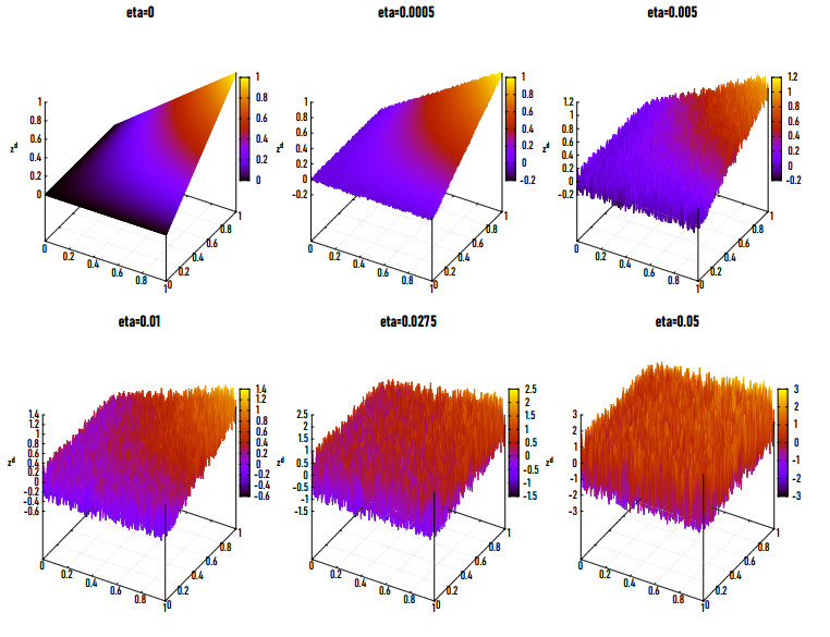
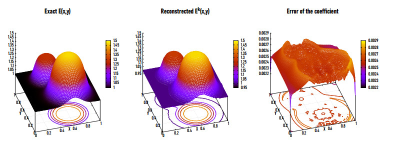
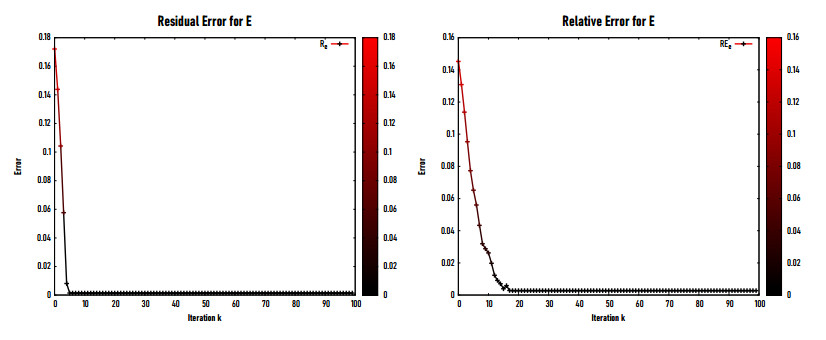
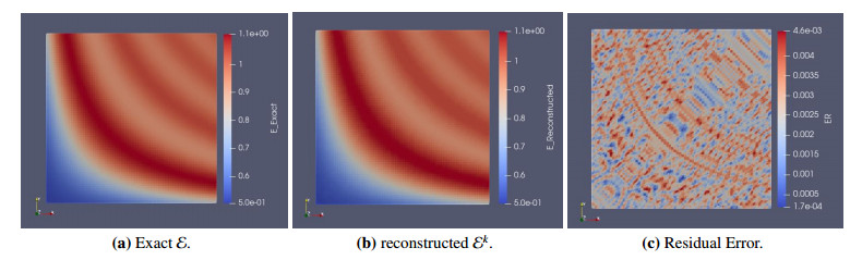
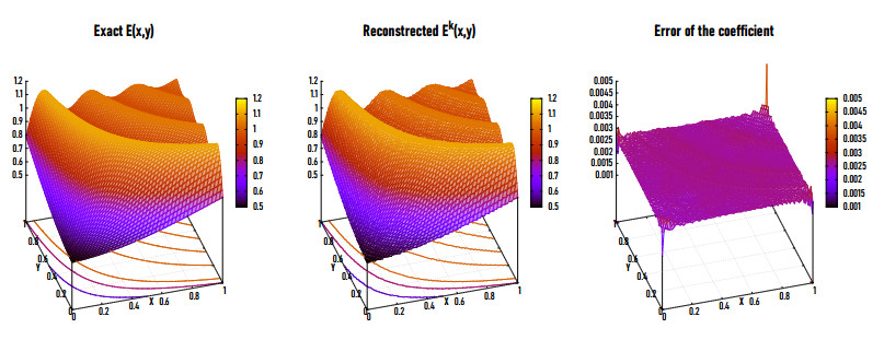
The present study focuses on reconstructing the Young's modulus for the elasticity imaging inverse problem. It is a very interesting and challenging problem encountered in tumor detection where the variation of the elastic properties of soft tissues allows to distinguish between normal and diseased tissues. The Levenberg-Marquardt method is used to treat this ill-posed inverse problem and the non-convex minimization is changed into a convex one. We get an explicit expression for computing the descent direction. The proposed technique with a constant and space dependant coefficients and for various real materials is examined. The obtained results of the 2D and 3D view for the reconstructed Young's modulus are agree with those of the exact coefficients. The proposed algorithm is implemented for different levels of noise in the data.
Citation: Talaat Abdelhamid, F. Khayat, H. Zayeni, Rongliang Chen. Levenberg-Marquardt method for identifying Young's modulus of the elasticity imaging inverse problem[J]. Electronic Research Archive, 2022, 30(4): 1532-1557. doi: 10.3934/era.2022079
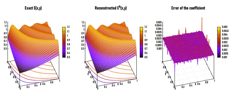
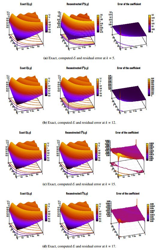
The present study focuses on reconstructing the Young's modulus for the elasticity imaging inverse problem. It is a very interesting and challenging problem encountered in tumor detection where the variation of the elastic properties of soft tissues allows to distinguish between normal and diseased tissues. The Levenberg-Marquardt method is used to treat this ill-posed inverse problem and the non-convex minimization is changed into a convex one. We get an explicit expression for computing the descent direction. The proposed technique with a constant and space dependant coefficients and for various real materials is examined. The obtained results of the 2D and 3D view for the reconstructed Young's modulus are agree with those of the exact coefficients. The proposed algorithm is implemented for different levels of noise in the data.

| [1] | J. E. Dennis, R. B. Schnabel, Numerical Methods for Unconstrained Optimization and Nonlinear Equations, Society for Industrial and Applied Mathematics, Philadelphia, 1996. |
| [2] | R. Fletcher, Practical Methods of Optimization, 2nd edition, Chichester, New York, 1987. |
| [3] |
K. Levenberg, A method for the solution of certain non-linear problems in least squares, Quart. Appl. Math., 2 (1944), 164–168. https://doi.org/10.1090/qam/10666 doi: 10.1090/qam/10666

|
| [4] |
D. W. Marquardt, An algorithm for least-squares estimation of nonlinear parameters, J. Soc. Ind. Appl. Math., 11 (1963), 431–441. https://doi.org/10.1137/0111030 doi: 10.1137/0111030
|
| [5] | C. T. Kelley, Iterative Methods for Optimization, Frontiers in applied mathematics, Philadelphia: SIAM, 1999. |
| [6] | N. Yamashita, M. Fukushima, On the Rate of Convergence of the Levenberg-Marquardt Method, Springer Vienna, (2001), 239–249. https://doi.org/10.1023/A:1013211030505 |
| [7] | M. I. A. Lourakis, A brief description of the levenberg-marquardt algorithm implemened by levmar, Found. Res. Technol., 4 (2005), 1–6. |
| [8] |
F. Facchinei, C. Kanzow, A nonsmooth inexact Newton method for the solution of large-scale nonlinear complementarity problems, Math. Program., 76 (1997), 493–512. https://doi.org/10.1007/BF02614395 doi: 10.1007/BF02614395
|
| [9] | D. P. Bertsekas, Dynamic Programming and Optimal Control, Mass: Athena Scientific, Belmont, 1995. |
| [10] | D. P. Bertsekas, Nonlinear Programming, 2nd edition, No. 4 in Athena scientific optimization and computation series, Massachusetts: Athena Scientific, Belmont, 2008. |
| [11] |
M. Hanke, A regularizing Levenberg-Marquardt scheme with applications to inverse groundwater filtration problems, Inverse Probl., 13 (1997), 79–95. https://doi.org/10.1088/0266-5611/13/1/007 doi: 10.1088/0266-5611/13/1/007
|
| [12] | F. Khayat, Identification of piecewise constant Robin coefficient for the Stokes problem using the Levenberg-Marquardt method, Comp. Appl. Math., 39 (2020), 185. |
| [13] |
J. Y. Fan, Y. X. Yuan, On the quadratic convergence of the Levenberg-Marquardt method without nonsingularity assumption, Computing, 74 (2005), 23–39. https://doi.org/10.1007/s00607-004-0083-1 doi: 10.1007/s00607-004-0083-1
|
| [14] |
D. Jiang, H. Feng, J. Zou, Quadratic convergence of Levenberg-Marquardt method for elliptic and parabolic inverse robin problems, ESAIM: M2AN, 52 (2018), 1085–1107. https://doi.org/10.1051/m2an/2018016 doi: 10.1051/m2an/2018016
|
| [15] |
N. Yamashita, M. Fukushima, The proximal point algorithm with genuine superlinear convergence for the monotone complementarity problem, SIAM J. Optim., 11 (2000), 364–379. https://doi.org/10.1137/S105262349935949X doi: 10.1137/S105262349935949X
|
| [16] |
Y. Mei, R. Fulmer, V. Raja, S. Wang, S. Goenezen, Estimating the non-homogeneous elastic modulus distribution from surface deformations, Int. J. Solids Struct., 83 (2016), 73–80. https://doi.org/10.1016/j.ijsolstr.2016.01.001 doi: 10.1016/j.ijsolstr.2016.01.001
|
| [17] |
K. Raghavan, A. Yagle, Forward and inverse problems in elasticity imaging of soft tissues, IEEE Trans. Nucl. Sci., 41 (1994), 1639–1648. https://doi.org/10.1109/23.322961 doi: 10.1109/23.322961
|
| [18] |
M. M. Doyley, P. M. Meaney, J. C. Bamber, Evaluation of an iterative reconstruction method for quantitative elastography, Phys. Med. Biol., 45 (2000), 1521–1540. https://doi.org/10.1088/0031-9155/45/6/309 doi: 10.1088/0031-9155/45/6/309
|
| [19] |
A. Constantinescu, On the identification of elastic moduli from displacement-force boundary measurements, Inverse Probl. Eng., 1 (1995), 293–313. https://doi.org/10.1080/174159795088027587 doi: 10.1080/174159795088027587
|
| [20] |
A. A. Oberai, N. H. Gokhale, G. R. Feijo, Solution of inverse problems in elasticity imaging using the adjoint method, Inverse Probl., 19 (2003), 297–313. https://doi.org/10.1088/0266-5611/19/2/304 doi: 10.1088/0266-5611/19/2/304
|
| [21] |
B. Jadamba, A. A. Khan, G. Rus, M. Sama, B. Winkler, A new convex inversion framework for parameter identification in saddle point problems with an application to the elasticity imaging inverse problem of predicting tumor location, SIAM J. Appl. Math., 74 (2014), 1486–1510. https://doi.org/10.1137/130928261 doi: 10.1137/130928261
|
| [22] | A. Arnold, S. Reichling, O. T. Bruhns, J. Mosler, Efficient computation of the elastography inverse problem by combining variational mesh adaption and a clustering technique, Phys. Med. Biol., 55 (2010), 2035–2056. |
| [23] |
T. Abdelhamid, R. Chen, M. M. Alam, Nonlinear conjugate gradient method for identifying Young's modulus of the elasticity imaging inverse problem, Inverse Probl. Sci. Eng., 29 (2021), 2165–2185. https://doi.org/10.1080/17415977.2021.1905638 doi: 10.1080/17415977.2021.1905638
|
| [24] | N. Mohammadi, M. M. Doyley, M. Cetin, A Statistical Framework for Model-Based Inverse Problems in Ultrasound Elastography, Pacific Grove, CA, USA: IEEE, 2020. https://doi.org/10.1109/IEEECONF51394.2020.9443450 |
| [25] |
M. A. Z. Raja, M. Shoaib, S. Hussain, K. S. Nisar, S. Islam, Computational intelligence of Levenberg-Marquardt backpropagation neural networks to study thermal radiation and Hall effects on boundary layer flow past a stretching sheet, Int. Commun. Heat Mass Transfer, 130 (2022), 105799. https://doi.org/10.1016/j.icheatmasstransfer.2021.105799 doi: 10.1016/j.icheatmasstransfer.2021.105799
|
| [26] | M. Shoaib, M. A. Z. Raja, G. Zubair, I. Farhat, K. S. Nisar, Z. Sabir, et al., Intelligent computing with Levenberg-Marquardt backpropagation neural networks for third-grade nanofluid over a stretched sheet with convective conditions, Arabian J. Sci. Eng., 2021, 1–19. |
| [27] |
H. Sung, J. Ferlay, R. L. Siegel, M. Laversanne, I. Soerjomataram, A. Jemal, et al., Global cancer statistics 2020: globocan estimates of incidence and mortality worldwide for 36 cancers in 185 countries, CA: Cancer J. Clin., 71 (2021), 209–249. https://doi.org/10.3322/caac.21660 doi: 10.3322/caac.21660
|
| [28] |
F. Bray, J. Ferlay, I. Soerjomataram, R. L. Siegel, L. A. Torre, A. Jemal, Global cancer statistics 2018: Globocan estimates of incidence and mortality worldwide for 36 cancers in 185 countries, CA: Cancer J. Clin., 68 (2018), 394–424. https://doi.org/10.3322/caac.21492 doi: 10.3322/caac.21492
|
| [29] | J. N. Reddy, An Introduction to the Finite Element Method, 3rd edition, McGraw-Hill series in mechanical engineering, McGraw-Hill Higher Education, New York, 2006. |
| [30] | Y. W. Kwon, H. Bang, The Finite Element Method Using MATLAB, 2nd edition, CRC mechanical engineering series, CRC Press, Boca Raton, 2000. |
| [31] |
F. Hecht, New development in FreeFem++, J. Numer. Math., 20 (2012), 251–266. https://doi.org/10.1515/jnum-2012-0013 doi: 10.1515/jnum-2012-0013
|
| [32] | A. H. Johnstone, CRC handbook of chemistry and physics, J. Chem. Technol. Biotechnol., 50 (2007), 294–295. |
| [33] | R. B. Ross, Metallic Materials Specification Handbook, 4th edition, Chapman & Hall, New York, 1992. |
| [34] | A. Nayar, The Metals Databook, New York, NY: McGraw-Hill, 1997. |
| [35] | D. R. Lide, CRC Handbook of Chemistry and Physics, 8th edition, CRC Press, Boca Raton, 1999. |
| [36] |
B. Jadamba, A. A. Khan, A. A. Oberai, M. Sama, First-order and second-order adjoint methods for parameter identification problems with an application to the elasticity imaging inverse problem, Inverse Probl. Sci. Eng., 25 (2017), 1768–1787. https://doi.org/10.1080/17415977.2017.1289195 doi: 10.1080/17415977.2017.1289195
|
Figures(18) / Tables(7)
Talaat Abdelhamid, F. Khayat, H. Zayeni, Rongliang Chen. Levenberg-Marquardt method for identifying Young's modulus of the elasticity imaging inverse problem[J]. Electronic Research Archive, 2022, 30(4): 1532-1557. doi: 10.3934/era.2022079


 DownLoad: