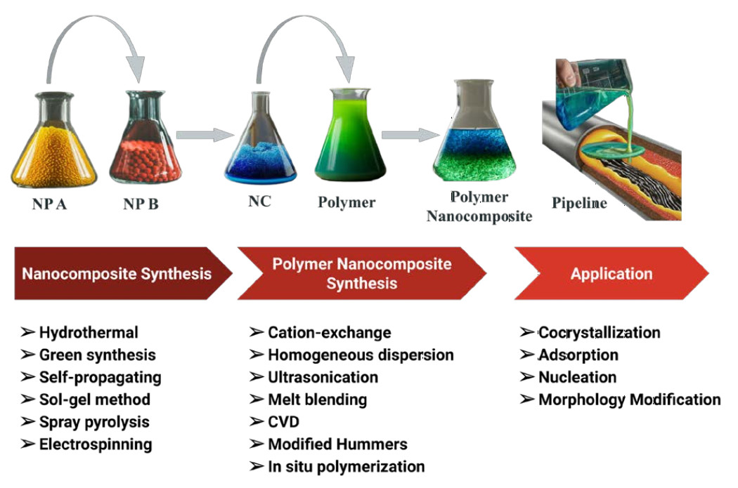
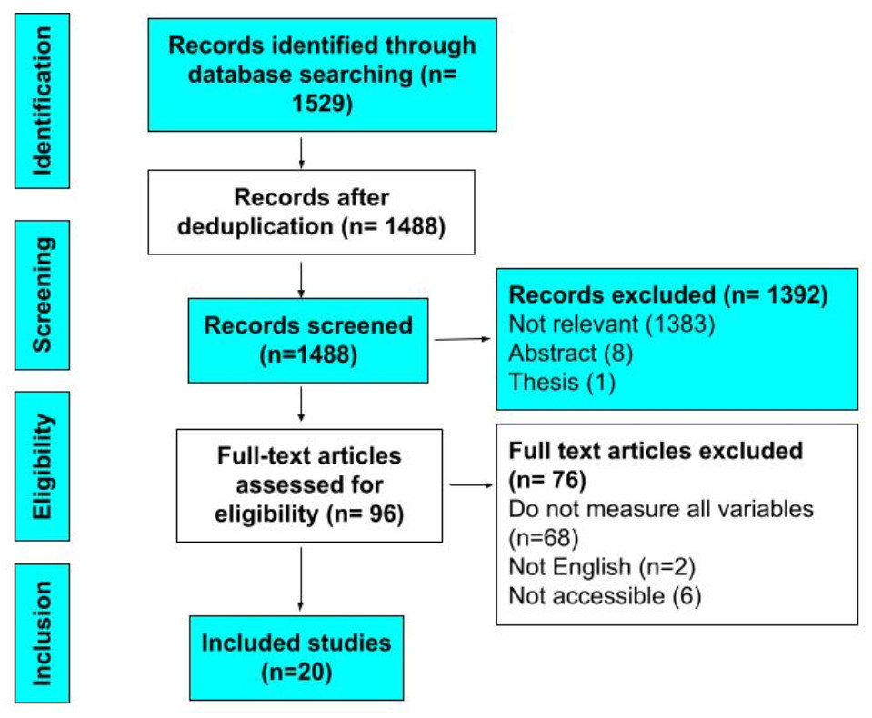
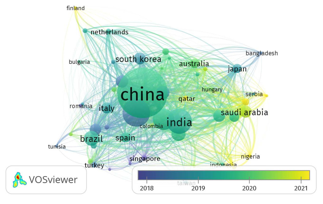
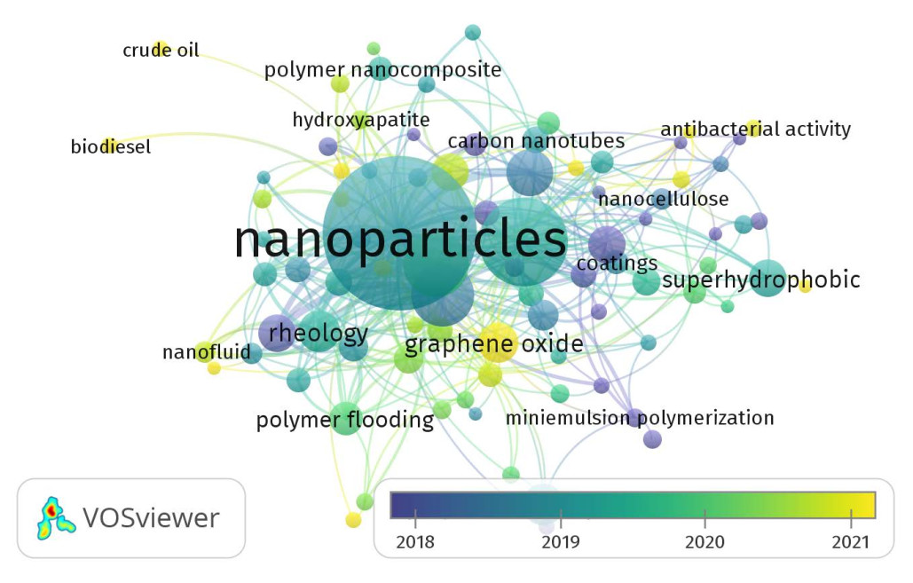
The extraction and utilization of crude oil are fundamental to global energy production, driving economies and fueling countless industries. However, wax deposition in pipelines and equipment creates several challenges, causing issues during the production, transportation, and refining of waxy crude oil. On the other hand, conventional chemicals such as alkylphenol ethoxylates (APEs) and volatile organic compounds (VOCs) used in the treatment have negative environmental and human health effects. Nanocomposites of polymers have emerged as promising solutions to mitigate wax damage. They represent a revolutionary class of nanocomposite hybridized polymer matrices. Moreover, to our knowledge, there has been a lack of comprehensive reviews of researchers who have combined and evaluated the effectiveness of these methods over the last decade. To gain a comprehensive understanding of the current state of knowledge and recognize emerging research trends, in this systematic review, we critically evaluated the published research on the role of polymer nanocomposites in the environmentally friendly management of wax deposition in crude oil systems. This review covers numerous topics, including (1) spatiotemporal distribution of research on polymer nanocomposites, (2) synthesis routes of millennium polymer nanocomposites, (3) reaction mechanisms for wax improvement, (4) common emerging trends in applications, (5) diverse polymer candidates for nanomaterials, (6) trending nanoparticle candidates for polymerization, and (7) future perspectives. However, further progress in understanding the effects of polymer nanocomposites on waxy crude oil is hindered by the lack of comparative studies on their reaction mechanisms and human health toxicity. However, despite these limitations, polymer nanocomposites continue to show great promise in addressing challenges related to waxy crude oil.
Citation: Abubakar Aji, Mysara Eissa Mohyaldinn, Hisham Ben Mahmud. The role of polymer nanocomposites in sustainable wax deposition control in crude oil systems - systematic review[J]. AIMS Environmental Science, 2025, 12(1): 16-52. doi: 10.3934/environsci.2025002
The extraction and utilization of crude oil are fundamental to global energy production, driving economies and fueling countless industries. However, wax deposition in pipelines and equipment creates several challenges, causing issues during the production, transportation, and refining of waxy crude oil. On the other hand, conventional chemicals such as alkylphenol ethoxylates (APEs) and volatile organic compounds (VOCs) used in the treatment have negative environmental and human health effects. Nanocomposites of polymers have emerged as promising solutions to mitigate wax damage. They represent a revolutionary class of nanocomposite hybridized polymer matrices. Moreover, to our knowledge, there has been a lack of comprehensive reviews of researchers who have combined and evaluated the effectiveness of these methods over the last decade. To gain a comprehensive understanding of the current state of knowledge and recognize emerging research trends, in this systematic review, we critically evaluated the published research on the role of polymer nanocomposites in the environmentally friendly management of wax deposition in crude oil systems. This review covers numerous topics, including (1) spatiotemporal distribution of research on polymer nanocomposites, (2) synthesis routes of millennium polymer nanocomposites, (3) reaction mechanisms for wax improvement, (4) common emerging trends in applications, (5) diverse polymer candidates for nanomaterials, (6) trending nanoparticle candidates for polymerization, and (7) future perspectives. However, further progress in understanding the effects of polymer nanocomposites on waxy crude oil is hindered by the lack of comparative studies on their reaction mechanisms and human health toxicity. However, despite these limitations, polymer nanocomposites continue to show great promise in addressing challenges related to waxy crude oil.

| [1] |
Elkatory MR, Soliman E, Nemr AE, et al. (2022) Mitigation and Remediation Technologies of Waxy Crude Oils' Deposition within Transportation Pipelines: A Review. Polymers 14. doi: 10.3390/polym14163231. doi: 10.3390/polym14163231

|
| [2] |
Mikulčić H, Baleta J, Wang X, et al. (2021) Green development challenges within the environmental management framework. J Environ Manage 277. doi: 10.1016/j.jenvman.2020.111477. doi: 10.1016/j.jenvman.2020.111477
|
| [3] |
Mishra P, Kiran NS, Romanholo Ferreira LF, et al. (2023) New insights into the bioremediation of petroleum contaminants: A systematic review. Chemosphere 326: 138391. doi: 10.1016/j.chemosphere.2023.138391. doi: 10.1016/j.chemosphere.2023.138391
|
| [4] |
Sharma R, Deka B, Mahto V, et al. (2022) Experimental investigation into the development and evaluation of ionic liquid and its graphene oxide nanocomposite as novel pour point depressants for waxy crude oil. J Pet Sci Eng 208: 109691. doi: 10.1016/j.petrol.2021.109691. doi: 10.1016/j.petrol.2021.109691
|
| [5] |
M'barki O, Clements J, Salazar L, et al. (2023) Impact of Paraffin Composition on the Interactions between Waxes, Asphaltenes, and Paraffin Inhibitors in a Light Crude Oil. Colloids Interfaces. doi: 10.3390/colloids7010013. doi: 10.3390/colloids7010013
|
| [6] |
Ismailova J, Abdukarimov A, Kabdushev A, et al. (2023) The implementation of fusion properties calculation to predict wax deposition. East-Eur J Enterp Technol. doi: 10.15587/1729-4061.2023.281657. doi: 10.15587/1729-4061.2023.281657
|
| [7] |
Elkatory MR, Hassaan M, Soliman E, et al. (2023) Influence of Poly (benzyl oleate-co-maleic anhydride) Pour Point Depressant with Di-Stearyl Amine on Waxy Crude Oil. Polymers 15. doi: 10.3390/polym15020306. doi: 10.3390/polym15020306
|
| [8] |
Ma Q, Wang C, Lu Y, et al. (2023) Water Droplets Tailored as Wax Crystal Carriers to Mitigate Wax Deposition of Emulsion. ACS Omega 8: 7546–7554. doi: 10.1021/acsomega.2c06809. doi: 10.1021/acsomega.2c06809
|
| [9] |
Mehrotra AK, Haj-Shafiei S, Ehsani S (2021) Predictions for wax deposition in a pipeline carrying paraffinic or 'waxy' crude oil from the heat-transfer approach. J Pipeline Sci Eng 1: 428–435. doi: 10.1016/j.jpse.2021.09.001. doi: 10.1016/j.jpse.2021.09.001
|
| [10] |
Bell E, Lu Y, Daraboina N, et al. (2021) Thermal methods in flow assurance: A review. J Nat Gas Sci Eng 88: 103798. doi: 10.1016/j.jngse.2021.103798. doi: 10.1016/j.jngse.2021.103798
|
| [11] |
Ali SI, Lalji SM, Awan Z, et al. (2023) Evaluation of different parameters affecting the performance of asphaltene controlling chemical additives in crude oils using multiple experimental approaches assisted with image processing technique. Geoenergy Sci Eng 225: 211676. doi: 10.1016/j.geoen.2023.211676. doi: 10.1016/j.geoen.2023.211676
|
| [12] |
Gao X, Huang Q, Yun Q, et al. (2024) Modeling wax deposit removal during pigging with foam pigs. Geoenergy Sci Eng 235: 212713. doi: 10.1016/j.geoen.2024.212713. doi: 10.1016/j.geoen.2024.212713
|
| [13] |
Gabayan RCM, Sulaimon A, Jufar S (2023) Application of Bio-Derived Alternatives for the Assured Flow of Waxy Crude Oil: A Review. Energies. doi: 10.3390/en16093652. doi: 10.3390/en16093652
|
| [14] |
Haldorai A, M S (2023) A Survey of Trends and Developments in Green Infrastructure Research. J Comput Nat Sci. doi: 10.53759/181x/jcns202303007. doi: 10.53759/181x/jcns202303007
|
| [15] |
Fung KCL, Dornelles HS, Varesche M, et al. (2023) From Wastewater Treatment Plants to the Oceans: A Review on Synthetic Chemical Surfactants (SCSs) and Perspectives on Marine-Safe Biosurfactants. Sustainability. doi: 10.3390/su151411436. doi: 10.3390/su151411436
|
| [16] |
Abidin MRSZ, Noh M, Moniruzzaman M, et al. (2023) Evaluation of Crude Oil Wax Dissolution Using a Hydrocarbon-Based Solvent in the Presence of Ionic Liquid. Processes. doi: 10.3390/pr11041112. doi: 10.3390/pr11041112
|
| [17] |
Kalidasan B, Pandey AK, Aljafari B, et al. (2023) Thermo-kinetic behaviour of green synthesized nanomaterial enhanced organic phase change material: Model fitting approach. J Environ Manage 348: 119439. doi: 10.1016/j.jenvman.2023.119439. doi: 10.1016/j.jenvman.2023.119439
|
| [18] |
Lin Q, Qin Y, Sun H, et al. (2023) SPE–UPLC–MS/MS for Determination of 36 Monomers of Alkylphenol Ethoxylates in Tea. Molecules 28. doi: 10.3390/molecules28073216. doi: 10.3390/molecules28073216
|
| [19] |
Cheng Y, Kong D, Ci M, et al. (2023) Oxidative Stress Effects of Multiple Pollutants in an Indoor Environment on Human Bronchial Epithelial Cells. Toxics 11. doi: 10.3390/toxics11030251. doi: 10.3390/toxics11030251
|
| [20] |
Zhou X, Zhou X, Wang C, et al. (2023) Environmental and human health impacts of volatile organic compounds: A perspective review. Chemosphere 313: 137489. doi: 10.1016/j.chemosphere.2022.137489. doi: 10.1016/j.chemosphere.2022.137489
|
| [21] |
Ruffolo F, Dinhof T, Murray L, et al. (2023) The Microbial Degradation of Natural and Anthropogenic Phosphonates. Molecules 28. doi: 10.3390/molecules28196863. doi: 10.3390/molecules28196863
|
| [22] |
Anbuchezhiyan G, Mubarak NM, Hussain Siddiqui MT, et al. (2024) Bo-derived waste neem to enriching reinforced hybrid composite for environmental remediation. Chemosphere 350: 141055. doi: 10.1016/j.chemosphere.2023.141055. doi: 10.1016/j.chemosphere.2023.141055
|
| [23] |
Saha A (2023) Polymer Nanocomposites: A Review on Recent Advances in the Field of Green Polymer Nanocomposites. Curr Nanosci 20: 706–716. doi: 10.2174/0115734137274950231113050300. doi: 10.2174/0115734137274950231113050300
|
| [24] |
Rashid MH-U-, Imran A, Susan M a. BH (2022) Green Polymer Nanocomposites in Automotive and Packaging Industries. Curr Pharm Biotechnol. doi: 10.2174/1389201023666220506111027. doi: 10.2174/1389201023666220506111027
|
| [25] |
Wypij M, Trzcińska-Wencel J, Golińska P, et al. (2023) The strategic applications of natural polymer nanocomposites in food packaging and agriculture: Chances, challenges, and consumers' perception. Front Chem 10. doi: 10.3389/fchem.2022.1106230. doi: 10.3389/fchem.2022.1106230
|
| [26] |
Shan P, Lu Y, Lu W, et al. (2022) Biodegradable and Light-Responsive Polymeric Nanoparticles for Environmentally Safe Herbicide Delivery. ACS Appl Mater Interfaces 11. doi: 10.1021/acsami.2c12106. doi: 10.1021/acsami.2c12106
|
| [27] |
López D, Ríos AA, Marín JD, et al. (2023) SiO2-Based Nanofluids for the Inhibition of Wax Precipitation in Production Pipelines. ACS Omega 8: 33289–33298. doi: 10.1021/acsomega.3c00802. doi: 10.1021/acsomega.3c00802
|
| [28] |
Ning X, Song X, Zhang S, et al. (2022) Insights into Flow Improving for Waxy Crude Oil Doped with EVA/SiO 2 Nanohybrids. ACS Omega 7: 5853–5863. doi: 10.1021/acsomega.1c05953. doi: 10.1021/acsomega.1c05953
|
| [29] | Ashkan M, Zainab H-D, Alimorad R (2021) Effect of nanoparticle modified polyacrylamide on wax deposition, crystallization and flow behavior of light and heavy crude oils. doi: https://doi.org/10.1080/01932691.2021.2010567. |
| [30] |
Jaberi I, Khosravi A, Rasouli S (2020) Graphene oxide-PEG: An effective anti-wax precipitation nano-agent in crude oil transportation. Upstream Oil Gas Technol 5: 100017. doi: 10.1016/j.upstre.2020.100017. doi: 10.1016/j.upstre.2020.100017
|
| [31] |
Ding H, Zhang H, Xie Q, et al. (2022) Synthesis and characterization of nano-SiO2 hybrid poly(methyl methacrylate) nanocomposites as novel wax inhibitor of asphalt binder. Colloids Surf Physicochem Eng Asp 653: 130023. doi: 10.1016/j.colsurfa.2022.130023. doi: 10.1016/j.colsurfa.2022.130023
|
| [32] |
Ghobashy MM, Alkhursani ShA, Alqahtani HA, et al. (2024) Gold nanoparticles in microelectronics advancements and biomedical applications. Mater Sci Eng B 301: 117191. doi: 10.1016/j.mseb.2024.117191. doi: 10.1016/j.mseb.2024.117191
|
| [33] |
Marmiroli M, Mussi F, Pagano L, et al. (2020) Cadmium sulfide quantum dots impact Arabidopsis thaliana physiology and morphology. Chemosphere 240: 124856. doi: 10.1016/j.chemosphere.2019.124856. doi: 10.1016/j.chemosphere.2019.124856
|
| [34] |
Umair M, Huma Zafar S, Cheema M, et al. (2024) New insights into the environmental application of hybrid nanoparticles in metal contaminated agroecosystem: A review. J Environ Manage 349: 119553. doi: 10.1016/j.jenvman.2023.119553. doi: 10.1016/j.jenvman.2023.119553
|
| [35] |
Alpandi AH, Husin H, Jeffri SI, et al. (2022) Investigation on Wax Deposition Reduction Using Natural Plant-Based Additives for Sustainable Energy Production from Penara Oilfield Malaysia Basin. ACS Omega 7: 30730–30745. doi: 10.1021/acsomega.2c01333. doi: 10.1021/acsomega.2c01333
|
| [36] |
Mohammadi S, Mahmoudi Alemi F (2021) Simultaneous Control of Formation and Growth of Asphaltene Solids and Wax Crystals Using Single-Walled Carbon Nanotubes: an Experimental Study under Real Oilfield Conditions. Energy Fuels 35: 14709–14724. doi: 10.1021/acs.energyfuels.1c02244. doi: 10.1021/acs.energyfuels.1c02244
|
| [37] |
El-Masry JF, Bou-Hamdan K, Abbas AH, et al. (2023) A Comprehensive Review on Utilizing Nanomaterials in Enhanced Oil Recovery Applications. Energies. doi: 10.3390/en16020691. doi: 10.3390/en16020691
|
| [38] |
Ali I, Shrivastava V (2021) Recent advances in technologies for removal and recovery of selenium from (waste)water: A systematic review. J Environ Manage 294: 112926. doi: 10.1016/j.jenvman.2021.112926. doi: 10.1016/j.jenvman.2021.112926
|
| [39] |
Mustapha A, Abdul-Rani AM, Saad N, et al. (2024) Ergonomic principles of road signs comprehension: A literature review. Transp Res Part F Traffic Psychol Behav 101: 279–305. doi: 10.1016/j.trf.2023.12.020. doi: 10.1016/j.trf.2023.12.020
|
| [40] |
Mostafa EM, Ghanem A, Hosny R, et al. (2024) In-situ upgrading of Egyptian heavy crude oil using matrix polymer carboxyl methyl cellulose/silicate graphene oxide nanocomposites. Sci Rep 14: 20985. doi: 10.1038/s41598-024-70843-3. doi: 10.1038/s41598-024-70843-3
|
| [41] |
Odutola TO (2023) A synergistic effect of zinc oxide nanoparticles and polyethylene butene improving the rheology of waxy crude oil. Pet Res 8: 217–225. doi: 10.1016/j.ptlrs.2023.01.004. doi: 10.1016/j.ptlrs.2023.01.004
|
| [42] | Shallsuku P (2023) Preparation and Application of Poly(methyl methacrylate)/alkyl imidazolium Modified Bentonite Nanocomposites for Deposition Mitigation of Nigerian Waxy Crude Oil. Int J Nat Pract Sci 5. |
| [43] |
Alves BF, Silva BKM, Silva CA, et al. (2023) Preparation and evaluation of polymeric nanocomposites based on EVA/montmorillonite, EVA/palygorskite and EVA/halloysite as pour point depressants and flow improvers of waxy systems. Fuel 333: 126540. doi: 10.1016/j.fuel.2022.126540. doi: 10.1016/j.fuel.2022.126540
|
| [44] |
Mahmoud T, Betiha MA (2021) Poly(octadecyl acrylate- co -vinyl neodecanoate)/Oleic Acid-Modified Nano-graphene Oxide as a Pour Point Depressant and an Enhancer of Waxy Oil Transportation. Energy Fuels 35: 6101–6112. doi: 10.1021/acs.energyfuels.1c00034. doi: 10.1021/acs.energyfuels.1c00034
|
| [45] |
Negi H, Sharma S, Singh RK (2021) Assessment of cellulose substituted with varying short/long, linear/branched acyl groups for inhibition of wax crystals growth in crude oil. J Ind Eng Chem 104: 458–467. doi: 10.1016/j.jiec.2021.08.043. doi: 10.1016/j.jiec.2021.08.043
|
| [46] | Rosdi MRH, Johary MDM, Ku KM, et al. (2020) Impact of Lateral Size of Graphene Oxide in Pour Point Depressant Composite on Wax Crystallisation of Model Oil. Pertanika J Sci Technol 28. |
| [47] |
Sharma R, Deka B, Mahto V, et al. (2019) Investigation into the Flow Assurance of Waxy Crude Oil by Application of Graphene-Based Novel Nanocomposite Pour Point Depressants. Energy Fuels 33: 12330–12345. doi: 10.1021/acs.energyfuels.9b03124. doi: 10.1021/acs.energyfuels.9b03124
|
| [48] |
Al‐Sabagh AM, Betiha MA, Osman DI, et al. (2018) Synthesis and characterization of nanohybrid of poly(octadecylacrylates derivatives)/montmorillonite as pour point depressants and flow improver for waxy crude oil. J Appl Polym Sci 136: 47333. doi: 10.1002/app.47333. doi: 10.1002/app.47333
|
| [49] |
Sharma R, Mahto V, Vuthaluru H (2019) Synthesis of PMMA/modified graphene oxide nanocomposite pour point depressant and its effect on the flow properties of Indian waxy crude oil. Fuel 235: 1245–1259. doi: 10.1016/j.fuel.2018.08.125. doi: 10.1016/j.fuel.2018.08.125
|
| [50] |
Zhao Z-B, Tai L, Zhang D-M, et al. (2017) Preparation of poly (octadecyl methacrylate)/silica-(3-methacryloxypropyl trimethoxysilane)/silica multi-layer core-shell nanocomposite with thermostable hydrophobicity and good viscosity break property. Chem Eng J 307: 891–896. doi: 10.1016/j.cej.2016.09.021. doi: 10.1016/j.cej.2016.09.021
|
| [51] |
Al-Sabagh AM, Betiha MA, Osman DI, et al. (2016) Preparation and Evaluation of Poly(methyl methacrylate)-Graphene Oxide Nanohybrid Polymers as Pour Point Depressants and Flow Improvers for Waxy Crude Oil. Energy Fuels 30: 7610–7621. doi: 10.1021/acs.energyfuels.6b01105. doi: 10.1021/acs.energyfuels.6b01105
|
| [52] |
Norrman J, Solberg A, Sjöblom J, et al. (2016) Nanoparticles for Waxy Crudes: Effect of Polymer Coverage and the Effect on Wax Crystallization. Energy Fuels 30: 5108–5114. doi: 10.1021/acs.energyfuels.6b00286. doi: 10.1021/acs.energyfuels.6b00286
|
| [53] |
Yao B, Li C, Yang F, et al. (2016) Structural properties of gelled Changqing waxy crude oil benefitted with nanocomposite pour point depressant. Fuel 184: 544–554. doi: 10.1016/j.fuel.2016.07.056. doi: 10.1016/j.fuel.2016.07.056
|
| [54] |
He C, Ding Y, Chen J, et al. (2016) Influence of the nano-hybrid pour point depressant on flow properties of waxy crude oil. Fuel 167: 40–48. doi: 10.1016/j.fuel.2015.11.031. doi: 10.1016/j.fuel.2015.11.031
|
| [55] |
Jia F, Jing W, Liu G, et al. (2020) Paraffin-based crude oil refining process unit-level energy consumption and CO2 emissions in China. J Clean Prod 255. doi: 10.1016/j.jclepro.2020.120347. doi: 10.1016/j.jclepro.2020.120347
|
| [56] |
Wang K-H, Su C, Lobonț O, et al. (2021) Whether crude oil dependence and CO2 emissions influence military expenditure in net oil importing countries? Energy Policy 153. doi: 10.1016/J.ENPOL.2021.112281. doi: 10.1016/J.ENPOL.2021.112281
|
| [57] | Fadairo A, Adeyemi G, Onyema O, et al. (2019) Formulation of Bio-Waste Derived Polymer and Its Application in Enhanced Oil Recovery. Day 2 Tue August 06 2019. doi: 10.2118/198750-MS. |
| [58] |
Grubert E, Hastings-Simon S (2022) Designing the mid-transition: A review of medium-term challenges for coordinated decarbonization in the United States. WIREs Clim Change 13: e768. doi: 10.1002/wcc.768. doi: 10.1002/wcc.768
|
| [59] |
Madurai Elavarasan R, Pugazhendhi R, Irfan M, et al. (2022) State-of-the-art sustainable approaches for deeper decarbonization in Europe – An endowment to climate neutral vision. Renew Sustain Energy Rev 159: 112204. doi: 10.1016/j.rser.2022.112204. doi: 10.1016/j.rser.2022.112204
|
| [60] |
Huo L, Guo J-F, Hu H, et al. (2022) Graphene Nanosheets as Lubricant Additives: Effects of Nature and Size on Lubricating Performance. Langmuir ACS J Surf Colloids. doi: 10.1021/acs.langmuir.2c01322. doi: 10.1021/acs.langmuir.2c01322
|
| [61] |
Li H, Shang Y, Zeng X, et al. (2022) Study on the Liquid-Liquid and Liquid-Solid Interfacial Behavior of Functionalized Graphene Oxide. Langmuir ACS J Surf Colloids. doi: 10.1021/acs.langmuir.1c02908. doi: 10.1021/acs.langmuir.1c02908
|
| [62] |
Xu Y, Wang Y, Wang T, et al. (2022) Demulsification of Heavy Oil-in-Water Emulsion by a Novel Janus Graphene Oxide Nanosheet: Experiments and Molecular Dynamic Simulations. Molecules 27. doi: 10.3390/molecules27072191. doi: 10.3390/molecules27072191
|
| [63] |
Said MNA, Hasbullah NA, Rosdi MRH, et al. (2023) Emulsion Polymerisation of Poly(Methyl Methacrylate)-Grafted-Graphene Oxide (PMMA-GO): Effect of Surfactant Concentration on Colloidal Stabilization. Mater Sci Forum 1102: 21–26. doi: 10.4028/p-Iqo7TL. doi: 10.4028/p-Iqo7TL
|
| [64] |
Itas YS, Suleiman AB, Ndikilar CE, et al. (2023) New trends in the hydrogen energy storage potentials of (8, 8) SWCNT and SWBNNT using optical adsorption spectra analysis: a DFT study. J Comput Electron 22: 1595–1605. doi: 10.1007/s10825-023-02093-x. doi: 10.1007/s10825-023-02093-x
|
| [65] | Xu L, Zhuk I, Sirak S (2023) Novel Modified Polycarboxylate Paraffin Inhibitor Blends Reduce C30+ Wax Deposits in South Texas. Day 1 Wed June 28 2023. doi: 10.2118/213853-ms. |
| [66] |
Sehn T, Meier MAR (2023) Structure-Property Relationships of Short Chain (Mixed) Cellulose Esters Synthesized in a DMSO/TMG/CO2 Switchable Solvent System. Biomacromolecules. doi: 10.1021/acs.biomac.3c00762. doi: 10.1021/acs.biomac.3c00762
|
| [67] |
Baharudin Ameer Naqiuddin, Risal Abdul Rahim, Zakaria Rozana, et al. (2022) Molecular Characteristics of Fatty Acid Methyl Ester (FAME) in Waxy Crude as Flow Improver. Chem Eng Trans 97: 295–300. doi: 10.3303/CET2297050. doi: 10.3303/CET2297050
|
| [68] |
Atta AM, El-Ghazawy RA, Morsy FA, et al. (2015) Adsorption of Polymeric Additives Based on Vinyl Acetate Copolymers as Wax Dispersant and Its Relevance to Polymer Crystallization Mechanisms. J Chem 2015: 1–8. doi: 10.1155/2015/683109. doi: 10.1155/2015/683109
|
| [69] |
Nazarychev V, Larin S, Lyulin A, et al. (2017) Atomistic Molecular Dynamics Simulations of the Initial Crystallization Stage in an SWCNT-Polyetherimide Nanocomposite. Polymers 9. doi: 10.3390/polym9100548. doi: 10.3390/polym9100548
|
| [70] |
Ahmad S, Nadeem S, Ullah N (2020) Entropy generation and temperature-dependent viscosity in the study of SWCNT–MWCNT hybrid nanofluid. Appl Nanosci 10: 5107–5119. doi: 10.1007/s13204-020-01306-0. doi: 10.1007/s13204-020-01306-0
|
| [71] |
Siddiq A, Ghobashy MM, El-Adasy AAAM, et al. (2024) Gamma radiation-induced grafting of poly(butyl acrylate) onto ethylene vinyl acetate copolymer for improved crude oil flowability. Sci Rep 14: 8863. doi: 10.1038/s41598-024-58521-w. doi: 10.1038/s41598-024-58521-w
|
| [72] |
Latif Z, Ali M, Lee E-J, et al. (2023) Thermal and Mechanical Properties of Nano-Carbon-Reinforced Polymeric Nanocomposites: A Review. J Compos Sci. doi: 10.3390/jcs7100441. doi: 10.3390/jcs7100441
|
| [73] |
Farha AH, Naim AAA, Mansour S (2020) Thermal Degradation of Polystyrene (PS) Nanocomposites Loaded with Sol Gel-Synthesized ZnO Nanorods. Polymers 12. doi: 10.3390/polym12091935. doi: 10.3390/polym12091935
|
| [74] |
D'Acierno F, Michal C, MacLachlan M (2023) Thermal Stability of Cellulose Nanomaterials. Chem Rev. doi: 10.1021/acs.chemrev.2c00816. doi: 10.1021/acs.chemrev.2c00816
|
| [75] |
Birinci E, Kaymakçı A (2023) Effect of Processing Technology, Nanomaterial and Coupling Agent Ratio on Some Physical, Mechanical, and Thermal Properties of Wood Polymer Nanocomposites. Forests. doi: 10.3390/f14051036. doi: 10.3390/f14051036
|
| [76] |
García-Muñoz MA, Valera-Zaragoza M, Aguirre-Cruz A, et al. (2023) Influence of compatibility in the EVA/starch/organoclay biodegradable nanocomposite on thermal properties and flame self-extinguishing behavior. Polym-Plast Technol Mater 62: 2318–2333. doi: 10.1080/25740881.2023.2258396. doi: 10.1080/25740881.2023.2258396
|
| [77] |
Dokuchaeva A, Vladimirov SV, Borodin VP, et al. (2023) Influence of Single-Wall Carbon Nanotube Suspension on the Mechanical Properties of Polymeric Films and Electrospun Scaffolds. Int J Mol Sci 24. doi: 10.3390/ijms241311092. doi: 10.3390/ijms241311092
|
| [78] |
Yusuff A, Bangwal D, Gbadamosi AO, et al. (2021) Kinetic and thermodynamic analysis of biodiesel and associated oil from Jatropha curcas L. during thermal degradation. Biomass Convers Biorefinery 13: 6121–6131. doi: 10.1007/s13399-021-01545-3. doi: 10.1007/s13399-021-01545-3
|
| [79] |
Zamri NN, Husin H (2023) Review on our point depressants for waxy crude oil issues. Platf J Eng 7: 2. doi: 10.61762/pajevol7iss1art21996. doi: 10.61762/pajevol7iss1art21996
|
| [80] |
Kamal R, Michel G, Ageez A, et al. (2023) Waste Plastic Nanomagnetite Pour Point Depressants for Heavy and Light Egyptian Crude Oil. ACS Omega 8: 3872–3881. doi: 10.1021/acsomega.2c06274. doi: 10.1021/acsomega.2c06274
|
| [81] |
Gbadamosi AO, Patil S, Kamal M, et al. (2022) Application of Polymers for Chemical Enhanced Oil Recovery: A Review. Polymers 14. doi: 10.3390/polym14071433. doi: 10.3390/polym14071433
|
| [82] |
Hassan YM, Guan B, Chuan LK, et al. (2022) Electromagnetically Modified Wettability and Interfacial Tension of Hybrid ZnO/SiO2 Nanofluids. Crystals. doi: 10.3390/cryst12020169. doi: 10.3390/cryst12020169
|
| [83] |
Liu Y, Sun Z, Jing G, et al. (2021) Synthesis of chemical grafting pour point depressant EVAL-GO and its effect on the rheological properties of Daqing crude oil. Fuel Process Technol 223: 107000. doi: 10.1016/j.fuproc.2021.107000. doi: 10.1016/j.fuproc.2021.107000
|
| [84] |
Rodríguez-Hernández A, Pérez-Martínez JD, Gallegos‐Infante J, et al. (2021) Rheological properties of ethyl cellulose-monoglyceride-candelilla wax oleogel vis-a-vis edible shortenings. Carbohydr Polym 252. doi: 10.1016/J.CARBPOL.2020.117171. doi: 10.1016/J.CARBPOL.2020.117171
|
| [85] |
Sun H, Lei X, Shen B, et al. (2018) Rheological properties and viscosity reduction of South China Sea crude oil. J Energy Chem 27: 1198–1207. doi: 10.1016/j.jechem.2017.07.023. doi: 10.1016/j.jechem.2017.07.023
|
| [86] |
Anuar A, M Saaid I, Tri Bhaskoro P, et al. (2023) Non-Newtonian Viscosity Behaviour Investigation for Malaysian Waxy Crude Oils and Impact to Wax Deposition Modelling. IIUM Eng J 24: 184–208. doi: 10.31436/iiumej.v24i2.2736. doi: 10.31436/iiumej.v24i2.2736
|
| [87] |
Olukanni D, Adegoke DA, Akinmejiwa AA, et al. (2023) Evaluation of Asphalt Produced from Waste Tyre and Polyethylene Terephthalate-Based Bitumen with Paraffin Wax as Rejuvenator. J Solid Waste Technol Manag. doi: 10.5276/jswtm/iswmaw/492/2023.270. doi: 10.5276/jswtm/iswmaw/492/2023.270
|
| [88] |
Li B, Guo Z, Zheng L, et al. (2024) A comprehensive review of wax deposition in crude oil systems: Mechanisms, influencing factors, prediction and inhibition techniques. Fuel 357: 129676. doi: 10.1016/j.fuel.2023.129676. doi: 10.1016/j.fuel.2023.129676
|
| [89] |
Dong H, Ma R, Zhao J, et al. (2023) Dynamic Behavior Analysis of Wax Crystals during Crude Oil Gelation. ACS Omega 8: 31085–31099. doi: 10.1021/acsomega.3c03021. doi: 10.1021/acsomega.3c03021
|
| [90] |
Ilyushin P, Vyatkin K, Kozlov A, et al. (2023) Study of the influence of dosing conditions of wax inhibitors on its efficiency using numerical simulation. Proc Inst Mech Eng Part E J Process Mech Eng. doi: 10.1177/09544089231158191. doi: 10.1177/09544089231158191
|
| [91] |
Wu H, Fahy W, Kim S, et al. (2020) Recent developments in polymers/polymer nanocomposites for additive manufacturing. Prog Mater Sci 111. doi: 10.1016/j.pmatsci.2020.100638. doi: 10.1016/j.pmatsci.2020.100638
|
| [92] |
Recio-Colmenares CL, Ortíz-Rios D, Pelayo-Vázquez JB, et al. (2022) Polystyrene Macroporous Magnetic Nanocomposites Synthesized through Deep Eutectic Solvent-in-Oil High Internal Phase Emulsions and Fe3O4 Nanoparticles for Oil Sorption. ACS Omega 7: 21763–21774. doi: 10.1021/acsomega.2c01836. doi: 10.1021/acsomega.2c01836
|
| [93] |
Saidi M, Safaripour M (2021) Ni–Mo nanoparticles stabilized by ether functionalized ionic polymer: A novel and efficient catalyst for hydrodeoxygenation of 4-methylanisole as a representative of lignin-derived pyrolysis bio-oils. Int J Hydrog Energy. doi: 10.1016/j.ijhydene.2020.10.274. doi: 10.1016/j.ijhydene.2020.10.274
|
| [94] |
Rana A, Frollini E, Thakur V (2021) Cellulose nanocrystals: Pretreatments, preparation strategies, and surface functionalization. Int J Biol Macromol. doi: 10.1016/j.ijbiomac.2021.05.119. doi: 10.1016/j.ijbiomac.2021.05.119
|
| [95] |
Chen J, Yuan N, Jiang D, et al. (2021) Octadecylamine and glucose-coderived hydrophobic carbon dots-modified porous silica for chromatographic separation. Chin Chem Lett. doi: 10.1016/J.CCLET.2021.04.052. doi: 10.1016/J.CCLET.2021.04.052
|
| [96] |
Castro-Landinez JF, Salcedo-Galán F, Medina-Perilla J (2021) Polypropylene/Ethylene—And Polar—Monomer-Based Copolymers/Montmorillonite Nanocomposites: Morphology, Mechanical Properties, and Oxygen Permeability. Polymers 13. doi: 10.3390/polym13050705. doi: 10.3390/polym13050705
|
| [97] |
Díez-Pascual A (2022) PMMA-Based Nanocomposites for Odontology Applications: A State-of-the-Art. Int J Mol Sci 23. doi: 10.3390/ijms231810288. doi: 10.3390/ijms231810288
|
| [98] |
Kumari S, Hussain A, Rao J, et al. (2023) Structural, mechanical and biological properties of PMMA-ZrO2 nanocomposites for denture applications. Mater Chem Phys 295: 127089. doi: 10.1016/j.matchemphys.2022.127089. doi: 10.1016/j.matchemphys.2022.127089
|
| [99] |
Lopes JA, Tsochatzis E (2023) Poly(ethylene terephthalate), Poly(butylene terephthalate), and Polystyrene Oligomers: Occurrence and Analysis in Food Contact Materials and Food. J Agric Food Chem. doi: 10.1021/acs.jafc.2c08558. doi: 10.1021/acs.jafc.2c08558
|
| [100] |
Li P, Chu Z, Chen Y, et al. (2021) One-pot and solvent-free synthesis of castor oil-based polyurethane acrylate oligomers for UV-curable coatings applications. Prog Org Coat 159. doi: 10.1016/J.PORGCOAT.2021.106398. doi: 10.1016/J.PORGCOAT.2021.106398
|
| [101] |
Saeaung K, Phusunti N, Phetwarotai W, et al. (2021) Catalytic pyrolysis of petroleum-based and biodegradable plastic waste to obtain high-value chemicals. Waste Manag 127: 101–111. doi: 10.1016/j.wasman.2021.04.024. doi: 10.1016/j.wasman.2021.04.024
|
| [102] |
Dmitrieva E, Anokhina T, Novitsky E, et al. (2022) Polymeric Membranes for Oil-Water Separation: A Review. Polymers 14. doi: 10.3390/polym14050980. doi: 10.3390/polym14050980
|
| [103] |
Betiha MA, Mahmoud T, Al-Sabagh A (2020) Effects of 4-vinylbenzyl trioctylphosphonium-bentonite containing poly(octadecylacrylate-co-1-vinyldodecanoate) pour point depressants on the cold flow characteristics of waxy crude oil. Fuel 282. doi: 10.1016/j.fuel.2020.118817. doi: 10.1016/j.fuel.2020.118817
|
| [104] |
Kazantsev O, Arifullin IR, Moikin AA, et al. (2021) Dependence of efficiency of polyalkyl acrylate-based pour point depressants on composition of crude oil. Egypt J Pet. doi: 10.1016/j.ejpe.2021.06.002. doi: 10.1016/j.ejpe.2021.06.002
|
| [105] |
Kojima S, Zhang L, Kumar C, et al. (2024) The effects of polyethylene glycol on the nucleation and growth of DNA-functionalized gold nanoparticles crystals. J Cryst Growth 640: 127740. doi: 10.1016/j.jcrysgro.2024.127740. doi: 10.1016/j.jcrysgro.2024.127740
|
| [106] |
Guo X, Wei K, Ni T, et al. (2024) Preparation and performance analysis of polyethylene glycol/epoxy resin composite phase change material. J Energy Storage 88: 111525. doi: 10.1016/j.est.2024.111525. doi: 10.1016/j.est.2024.111525
|
| [107] |
Tang J, Liu S, Liu W, et al. (2023) Comparative study on tribological performance and mechanism of eco-friendly solvent-free covalent MXene nanofluids in glycerin and polyethylene glycol. Tribol Int 190: 109051. doi: 10.1016/j.triboint.2023.109051. doi: 10.1016/j.triboint.2023.109051
|
| [108] |
Zhao X, Li P, Mo F, et al. (2024) Copolyester toughened poly(lactic acid) biodegradable material prepared by in situ formation of polyethylene glycol and citric acid. RSC Adv 14: 11027–11036. doi: 10.1039/d4ra00757c. doi: 10.1039/d4ra00757c
|
| [109] |
Sarac BA, Wordsworth M, Schmucker RW (2024) Polyethylene Glycol Fusion and Nerve Repair Success: Practical Applications. J Hand Surg Glob Online. doi: 10.1016/j.jhsg.2024.01.016. doi: 10.1016/j.jhsg.2024.01.016
|
| [110] |
Odutola TO, Allen BE (2023) The effect of polyethylene butene (PEB) and xylene on the shear stress of Niger delta crude oil. Glob J Eng Technol Adv. doi: 10.30574/gjeta.2023.14.3.0054. doi: 10.30574/gjeta.2023.14.3.0054
|
| [111] |
Pettignano A, Charlot A, Fleury E (2019) Carboxyl-functionalized derivatives of carboxymethyl cellulose: towards advanced biomedical applications. Polym Rev 59: 510–560. doi: 10.1080/15583724.2019.1579226. doi: 10.1080/15583724.2019.1579226
|
| [112] |
Osman WM, Ibrahim AA, Karma AB, et al. (2023) Design Process of CSTR for Production Carboxyl Methyl Cellulose. Int Res J Innov Eng Technol. doi: 10.47001/irjiet/2023.702004. doi: 10.47001/irjiet/2023.702004
|
| [113] |
Negi H, Sharma S, Singh R (2021) Assessment of cellulose substituted with varying short/long, linear/branched acyl groups for inhibition of wax crystals growth in crude oil. J Ind Eng Chem. doi: 10.1016/j.jiec.2021.08.043. doi: 10.1016/j.jiec.2021.08.043
|
| [114] |
Ahmed J, Rashed MA, Faisal M, et al. (2021) Novel SWCNTs-mesoporous silicon nanocomposite as efficient non-enzymatic glucose biosensor. Appl Surf Sci. doi: 10.1016/J.APSUSC.2021.149477. doi: 10.1016/J.APSUSC.2021.149477
|
| [115] |
Xiao X, Y Z, L Z, et al. (2022) Photoluminescence and Fluorescence Quenching of Graphene Oxide: A Review. Nanomater Basel Switz 12. doi: 10.3390/nano12142444. doi: 10.3390/nano12142444
|
| [116] |
Sable S, Mandal DK, Ahuja S, et al. (2019) Biodegradation kinetic modeling of oxo-biodegradable polypropylene/polylactide/nanoclay blends and composites under controlled composting conditions. J Environ Manage 249: 109186. doi: 10.1016/j.jenvman.2019.06.087. doi: 10.1016/j.jenvman.2019.06.087
|
| [117] |
Nazarahari M, Manshad AK, Ali M, et al. (2021) Impact of a novel biosynthesized nanocomposite (SiO2@Montmorilant@Xanthan) on wettability shift and interfacial tension: Applications for enhanced oil recovery. Fuel 298. doi: 10.1016/J.FUEL.2021.120773. doi: 10.1016/J.FUEL.2021.120773
|
| [118] |
Nagajyothi PC, Muthuraman P, Tettey CO, et al. (2021) In vitro anticancer activity of eco-friendly synthesized ZnO/Ag nanocomposites. Ceram Int 47: 34940–34948. doi: 10.1016/j.ceramint.2021.09.035. doi: 10.1016/j.ceramint.2021.09.035
|
| [119] |
Samavati A, Samavati Z, Ismail AF, et al. (2021) Multi aspect investigation of crude oil concentration detecting via optical fiber sensor coated with ZnO/Ag nano-heterostructure. Measurement 167: 108171. doi: 10.1016/j.measurement.2020.108171. doi: 10.1016/j.measurement.2020.108171
|
| [120] |
Luo C (2023) Organic electrode materials and carbon/small-sulfur composites for affordable, lightweight and sustainable batteries. Chem Commun. doi: 10.1039/d3cc02652c. doi: 10.1039/d3cc02652c
|
| [121] |
Alves L, Ferraz E, Gamelas J (2019) Composites of nanofibrillated cellulose with clay minerals: A review. Adv Colloid Interface Sci 272. doi: 10.1016/j.cis.2019.101994. doi: 10.1016/j.cis.2019.101994
|
| [122] |
Zou R, Xu J, Kuffner S, et al. (2019) Spherical Poly(vinyl imidazole) Brushes Loading Nickel Cations as Nanocatalysts for Aquathermolysis of Heavy Crude Oil. Energy Fuels. doi: 10.1021/ACS.ENERGYFUELS.8B03964. doi: 10.1021/ACS.ENERGYFUELS.8B03964
|
| [123] |
Zhang X, Shi Q, Luo L, et al. (2021) Research Progress on the Phase Change Materials for Cold Thermal Energy Storage. Energies. doi: 10.3390/en14248233. doi: 10.3390/en14248233
|
| [124] |
Rashid AA, Khan S, Al‐Ghamdi SG, et al. (2021) Additive manufacturing of polymer nanocomposites: Needs and challenges in materials, processes, and applications. J Mater Res Technol 14: 910–941. doi: 10.1016/J.JMRT.2021.07.016. doi: 10.1016/J.JMRT.2021.07.016
|
| [125] |
Lammari N, Louaer O, Méniai A, et al. (2020) Encapsulation of Essential Oils via Nanoprecipitation Process: Overview, Progress, Challenges and Prospects. Pharmaceutics 12. doi: 10.3390/pharmaceutics12050431. doi: 10.3390/pharmaceutics12050431
|
| [126] |
Hauser M, Li G, Nowack B (2019) Environmental hazard assessment for polymeric and inorganic nanobiomaterials used in drug delivery. J Nanobiotechnology 17. doi: 10.1186/s12951-019-0489-8. doi: 10.1186/s12951-019-0489-8
|
| [127] |
Hosseini H, Zirakjou A, Mcclements D, et al. (2021) Removal of methylene blue from wastewater using ternary nanocomposite aerogel systems: Carboxymethyl cellulose grafted by polyacrylic acid and decorated with graphene oxide. J Hazard Mater 421. doi: 10.1016/j.jhazmat.2021.126752. doi: 10.1016/j.jhazmat.2021.126752
|
| [128] |
Rai P, Lee J, Brown RJC, et al. (2021) Environmental fate, ecotoxicity biomarkers, and potential health effects of micro- and nano-scale plastic contamination. J Hazard Mater 403. doi: 10.1016/J.JHAZMAT.2020.123910. doi: 10.1016/J.JHAZMAT.2020.123910
|
Figures(6) / Tables(1)

Abubakar Aji, Mysara Eissa Mohyaldinn, Hisham Ben Mahmud. The role of polymer nanocomposites in sustainable wax deposition control in crude oil systems - systematic review[J]. AIMS Environmental Science, 2025, 12(1): 16-52. doi: 10.3934/environsci.2025002


 DownLoad: