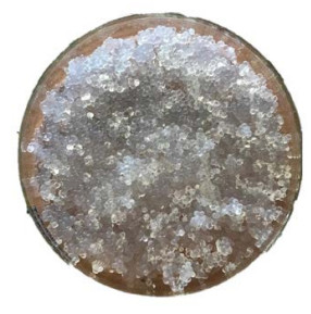
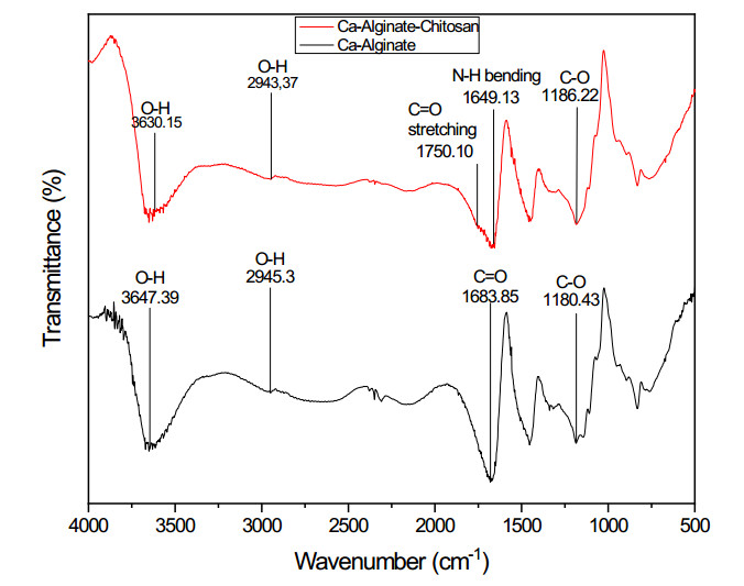
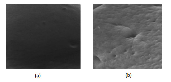
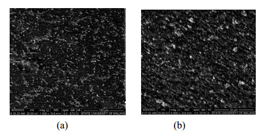
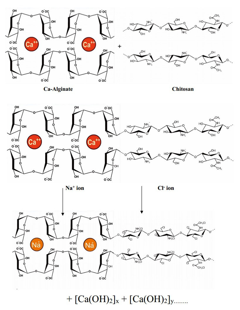
Initial research was focused on the production of calcium-based alginate-chitosan membranes from coral skeletons collected from the Gulf of Prigi. The coral skeleton's composition was analyzed using XRF, revealing a calcium oxide content ranging from 90.86% to 93.41%. These membranes showed the significant potential for salt adsorption, as evidenced by FTIR analysis, which showed the presence of functional groups such as -OH, C = O, C-O, and N-H involved in the NaCl binding process. SEM analysis showed the particle size diameter of 185.96 nm, indicating a relatively rough and porous morphology. Under optimized conditions, the resulting calcium-based alginate-chitosan membrane achieved 40.5% Na+ and 48.39% Cl- adsorptions, using 13.3 mL of 2% (w/v) chitosan and 26.6 mL of 2% (w/v) alginate with a 40-minutes contact time. The subsequent we applied for the desalination potential of calcium alginate, revealing the efficient reduction of NaCl levels in seawater. The calcium of coral skeletons collected was 90.86% and 93.41% before and after calcination, respectively, affirming the dominant calcium composition suitable for calcium alginate production. We identified an optimal 8-minute contact time for calcium alginate to effectively absorb NaCl, resulting in an 88.17% and 50% for Na+ and Cl- absorptions. We applied the addition of chitosan into calcium-alginate membranes and its impact on enhancing salt adsorption efficiency for seawater desalination.
Citation: Anugrah Ricky Wijaya, Alif Alfarisyi Syah, Dhea Chelsea Hana, Helwani Fuadi Sujoko Putra. Addition of chitosan to calcium-alginate membranes for seawater NaCl adsorption[J]. AIMS Environmental Science, 2024, 11(1): 75-89. doi: 10.3934/environsci.2024005
Initial research was focused on the production of calcium-based alginate-chitosan membranes from coral skeletons collected from the Gulf of Prigi. The coral skeleton's composition was analyzed using XRF, revealing a calcium oxide content ranging from 90.86% to 93.41%. These membranes showed the significant potential for salt adsorption, as evidenced by FTIR analysis, which showed the presence of functional groups such as -OH, C = O, C-O, and N-H involved in the NaCl binding process. SEM analysis showed the particle size diameter of 185.96 nm, indicating a relatively rough and porous morphology. Under optimized conditions, the resulting calcium-based alginate-chitosan membrane achieved 40.5% Na+ and 48.39% Cl- adsorptions, using 13.3 mL of 2% (w/v) chitosan and 26.6 mL of 2% (w/v) alginate with a 40-minutes contact time. The subsequent we applied for the desalination potential of calcium alginate, revealing the efficient reduction of NaCl levels in seawater. The calcium of coral skeletons collected was 90.86% and 93.41% before and after calcination, respectively, affirming the dominant calcium composition suitable for calcium alginate production. We identified an optimal 8-minute contact time for calcium alginate to effectively absorb NaCl, resulting in an 88.17% and 50% for Na+ and Cl- absorptions. We applied the addition of chitosan into calcium-alginate membranes and its impact on enhancing salt adsorption efficiency for seawater desalination.

| [1] |
Bibi A, Ur-Rehman S, Akhtar T, et al. (2020) Effective removal of carcinogenic dye from aqueous solution by using alginate-based nanocomposites. Desalin Water Treatt 208: 386–398. https://doi.org/10.5004/dwt.2020.26432 doi: 10.5004/dwt.2020.26432

|
| [2] |
Millero FJ, Feistel R, Wright DG, et al. (2008) The composition of Standard Seawater and the definition of the Reference-Composition Salinity Scale. Deep-Sea Res Part Ⅰ-Oceanogr Res Pap 55: 50–72. https://doi.org/10.1016/j.dsr.2007.10.001 doi: 10.1016/j.dsr.2007.10.001
|
| [3] |
Armid A, Shinjo R, Takwir A, et al. (2021) Spatial distribution and pollution assessment of trace elements Pb, Cu, Ni, Fe and as in the surficial water of Staring Bay, Indonesia. J Braz Chem Soc 32: 299–310. https://doi.org/10.21577/0103-5053.20200180 doi: 10.21577/0103-5053.20200180
|
| [4] | Wijaya AR, Khoerunnisa F, Armid A, et al. (2022) The best-modified BCR and Tessier with microwave-assisted methods for leaching of Cu/Zn and their δ65Cu/δ66Zn for tracing sources in marine sediment fraction. Environ Technol Innov 28. |
| [5] |
Wijaya AR, Kusumaningrum IK, Hakim L, et al. (2022) Road-side dust from central Jakarta, Indonesia: Assessment of metal(loid) content, mineralogy, and bioaccessibility. Environ Technol Innov 28: 102934. https://doi.org/10.1016/j.eti.2022.102934 doi: 10.1016/j.eti.2022.102934
|
| [6] | Lachish U (2007) Optimizing the Efficiency of Reverse Osmosis Seawater Desalination. 1–17. |
| [7] |
Honarparvar S, Zhang X, Chen T, et al. (2021) Frontiers of membrane desalination processes for brackish water treatment: A review. Membranes 11. https://doi.org/10.3390/membranes11040246 doi: 10.3390/membranes11040246
|
| [8] |
Piekarska K, Sikora M, Owczarek M, et al. (2023) Chitin and Chitosan as Polymers of the Future—Obtaining, Modification, Life Cycle Assessment and Main Directions of Application. Polymers 15. https://doi.org/10.3390/polym15040793 doi: 10.3390/polym15040793
|
| [9] |
Zhang H, Li X, Zheng S, et al. (2023) The coral-inspired steam evaporator for efficient solar desalination via porous and thermal insulation bionic design. SmartMat 4: 1–12. https://doi.org/10.1002/smm2.1175 doi: 10.1002/smm2.1175
|
| [10] |
Cao DQ, Tang K, Zhang WY, et al. (2023) Calcium Alginate Production through Forward Osmosis with Reverse Solute Diffusion and Mechanism Analysis. Membranes 13: 1–15. https://doi.org/10.3390/membranes13020207 doi: 10.3390/membranes13020207
|
| [11] |
Nakayama R ichi, Takamatsu Y, Namiki N (2020) Multiphase calcium alginate membrane composited with cellulose nanofibers for selective mass transfer. SN Appl Sci 2: 1–7. https://doi.org/10.1007/s42452-020-03532-1 doi: 10.1007/s42452-020-03532-1
|
| [12] |
Long Q, Zhang Z, Qi G, et al. (2020) Fabrication of Chitosan Nanofiltration Membranes by the Film Casting Strategy for Effective Removal of Dyes/Salts in Textile Wastewater. ACS Sustain Chem Eng 8: 2512–2522. https://doi.org/10.1021/acssuschemeng.9b07026 doi: 10.1021/acssuschemeng.9b07026
|
| [13] |
Nalatambi S, Oh KS, Yoon LW (2021) Fabrication technique of composite chitosan/alginate membrane module for greywater treatment. J Physics Conf Ser 2120. https://doi.org/10.1088/1742-6596/2120/1/012037 doi: 10.1088/1742-6596/2120/1/012037
|
| [14] |
Benettayeb A, Ghosh S, Usman M, et al. (2022) Some Well-Known Alginate and Chitosan Modifications Used in Adsorption: A Review. Water 14: 1–26. https://doi.org/10.3390/w14091353 doi: 10.3390/w14091353
|
| [15] |
Thanakkasaranee S, Sadeghi K, Lim IJ, et al. (2020) Effects of incorporating calcined corals as natural antimicrobial agent into active packaging system for milk storage. Mater Sci Eng C 111: 110781. https://doi.org/10.1016/j.msec.2020.110781 doi: 10.1016/j.msec.2020.110781
|
| [16] |
Shahid MK, Mainali B, Rout PR, et al. (2023) A Review of Membrane-Based Desalination Systems Powered by Renewable Energy Sources. Water 15. https://doi.org/10.3390/w15030534 doi: 10.3390/w15030534
|
| [17] |
Kosanović C, Fermani S, Falini G, et al. (2017) Crystallization of calcium carbonate in alginate and xanthan hydrogels. Crystals 7: 1–15. https://doi.org/10.3390/cryst7120355 doi: 10.3390/cryst7120355
|
| [18] |
Milita S, Zaquin T, Fermani S, et al. (2023) Assembly of the Intraskeletal Coral Organic Matrix during Calcium Carbonate Formation. Cryst Growth Des 23: 5801–5811. https://doi.org/10.1021/acs.cgd.3c00401 doi: 10.1021/acs.cgd.3c00401
|
| [19] |
Goffredo S, Vergni P, Reggi M, et al. (2011) The skeletal organic matrix from Mediterranean coral Balanophyllia Europaea influences calcium carbonate precipitation. PLoS ONE 6. https://doi.org/10.1371/journal.pone.0022338 doi: 10.1371/journal.pone.0022338
|
| [20] |
Suci CW, Wijaya AR (2020) Analysis of fe in coral reefs for monitoring environmental areas of prigi coast waters using the tessier-microwave method. IOP Conf Ser Mater Sci Eng 833. https://doi.org/10.1088/1757-899X/833/1/012046 doi: 10.1088/1757-899X/833/1/012046
|
| [21] |
Suci CW, Wijaya AR, Santoso A, et al. (2020) Fe leaching in the sludge sediment of the prigi beach with tessier-microwave method. AIP Conference Proceedings 2231. https://doi.org/10.1063/5.0002589 doi: 10.1063/5.0002589
|
| [22] |
Pavoni JMF, Luchese CL, Tessaro IC (2019) Impact of acid type for chitosan dissolution on the characteristics and biodegradability of cornstarch/chitosan based films. Int J Biol Macromol 138: 693–703. https://doi.org/10.1016/j.ijbiomac.2019.07.089 doi: 10.1016/j.ijbiomac.2019.07.089
|
| [23] |
Daemi H, Barikani M (2012) Synthesis and characterization of calcium alginate nanoparticles, sodium homopolymannuronate salt and its calcium nanoparticles. Sci Iran 19: 2023–2028. https://doi.org/10.1016/j.scient.2012.10.005 doi: 10.1016/j.scient.2012.10.005
|
| [24] | Grossi A, De Laia S, De Souza E, et al. (2014) a Study of Sodium Alginate and Calcium Chloride Interaction Through Films for Intervertebral Disc Regeneration Uses. 21o CBECIMAT - Congresso Brasileiro de Engenharia e Ciência dos Materiais 7341–7348. |
| [25] |
Venkatesan J, Bhatnagar I, Kim SK (2014) Chitosan-alginate biocomposite containing fucoidan for bone tissue engineering. Mar Drugs 12: 300–316. https://doi.org/10.3390/md12010300 doi: 10.3390/md12010300
|
| [26] |
Tang S, Yang J, Lin L, et al. (2020) Construction of physically crosslinked chitosan/sodium alginate/calcium ion double-network hydrogel and its application to heavy metal ions removal. Chem Eng J 393: 124728. https://doi.org/10.1016/j.cej.2020.124728 doi: 10.1016/j.cej.2020.124728
|
| [27] |
Hamedi H, Moradi S, Tonelli AE, et al. (2019) Preparation and characterization of chitosan–Alginate polyelectrolyte complexes loaded with antibacterial thyme oil nanoemulsions. Appl Sci 9. https://doi.org/10.3390/app9183933 doi: 10.3390/app9183933
|
| [28] |
Permanadewi I, Kumoro AC, Wardhani DH, et al. (2021) Analysis of Temperature Regulation, Concentration, and Stirring Time at Atmospheric Pressure to Increase Density Precision of Alginate Solution. Teknik 42: 29–34. https://doi.org/10.14710/teknik.v42i1.35994 doi: 10.14710/teknik.v42i1.35994
|
| [29] |
Lawrie G, Keen I, Drew B, et al. (2007) Interactions between alginate and chitosan biopolymers characterized using FTIR and XPS. Biomacromolecules 8: 2533–2541. https://doi.org/10.1021/bm070014y doi: 10.1021/bm070014y
|
| [30] |
Niculescu AG, Grumezescu AM (2022) Applications of Chitosan-Alginate-Based Nanoparticles— An Up-to-Date Review. Nanomaterials 12. https://doi.org/10.3390/nano12020186 doi: 10.3390/nano12020186
|
| [31] |
Rina Tri Vidia Ningsih, Anugrah Ricky Wijaya, Aman Santoso Aman M (2023) Chitosan membrane modification using silica prigi Bay for Na+ ion adsorption. AIP Conf Proc 2634: 020014. https://doi.org/10.1063/5.0111964 doi: 10.1063/5.0111964
|

Figures(6) / Tables(6)

Anugrah Ricky Wijaya, Alif Alfarisyi Syah, Dhea Chelsea Hana, Helwani Fuadi Sujoko Putra. Addition of chitosan to calcium-alginate membranes for seawater NaCl adsorption[J]. AIMS Environmental Science, 2024, 11(1): 75-89. doi: 10.3934/environsci.2024005


 DownLoad: