Treatment of greywater by Electrocoagulation process coupled with sand bed filter and activated carbon adsorption process in continuous mode

Prajakta Waghe; Khalid Ansari; Mohammad Hadi Dehghani; Tripti Gupta; Aniket Pathade; Charuta Waghmare; Prajakta Waghe; Khalid Ansari; Mohammad Hadi Dehghani; Tripti Gupta; Aniket Pathade; Charuta Waghmare

doi:10.3934/environsci.2024004

AIMS Environmental Science

2024, Volume 11, Issue 1: 57-74. doi: 10.3934/environsci.2024004

Previous Article Next Article

Research article Special Issues

Treatment of greywater by Electrocoagulation process coupled with sand bed filter and activated carbon adsorption process in continuous mode

1.
Department of Chemistry, Yeshwantrao Chavan College of Engineering, Nagpur, India, 441110
2.
Department of Civil Engineering, Yeshwantrao Chavan College of Engineering, Nagpur, India, 441110
3.
Department of Environmental Health Engineering, School of Public Health, Tehran University of Medical Sciences, Tehran, Iran
4.
Center for Solid Waste Research, Institute for Environmental Research, Tehran University Medical Sciences, Tehran, Iran
5.
Department of Civil Engineering, Shri Ramdeobaba College of Engineering and Management, Nagpur, India, 440013
6.
Research Consultant, Directorate of Research, Jawaharlal Nehru Medical College, Datta Meghe Institute of Higher Education and Research, Wardha, India, 442107
^†: Author Contributed Equally with First Author

Received: 30 October 2023 Revised: 20 December 2023 Accepted: 24 January 2024 Published: 05 February 2024

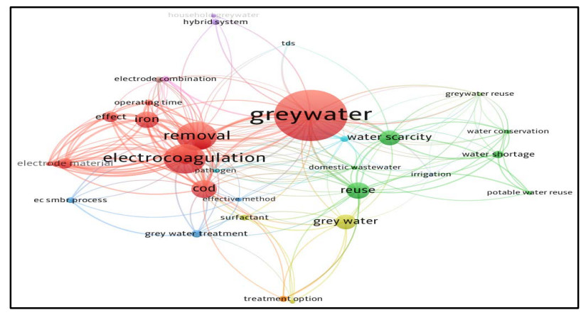
Worldwide population growth and consumerism have elevated the water pollution problem to the top of the environmental priority list, with severe consequences for public health, particularly in agricultural countries such as India, where water scarcity is a big challenge. Hence, greywater has the potential to be one of the most sustainable options to meet the growing need for freshwater with satisfying treatment options. This study focused on the assessment of electrocoagulation coupled with the filtration and adsorption processes in continuous modes and different electrode arrangements including (Al-Fe-Al-Fe), (Fe-Al-Fe-Al), (Al-Al-Al-Al) and (Fe-Fe-Fe-Fe) to investigate the effect of specific flow rates (i.e., 0.05 and 0.1 liters per minute) on the removal efficiency. The findings show that a 0.05 lit/min flow rate produces a higher removal efficiency approximately between 85 to 90% with an energy consumption of between 0.5 to 4.75 KWh/m³ as compared to the 75 to 85% removal efficiency and 0.4 to 4 KWh/m³ energy consumption at a flow rate of 0.1 lit/min. The operational cost is variable and mainly depends upon the energy consumption; moreover, it was found that the optimal results and economy variation shown by the electrode assembly of Al-Fe-Al-Fe was between 20 to 22 Indian rupees at a 24 volt current density and in each combination of electrodes.
- electrocoagulation process,
- sand bed filter,
- activated carbon,
- continuous mode,
- greywater
Citation: Prajakta Waghe, Khalid Ansari, Mohammad Hadi Dehghani, Tripti Gupta, Aniket Pathade, Charuta Waghmare. Treatment of greywater by Electrocoagulation process coupled with sand bed filter and activated carbon adsorption process in continuous mode[J]. AIMS Environmental Science, 2024, 11(1): 57-74. doi: 10.3934/environsci.2024004

Related Papers:

Abstract

Worldwide population growth and consumerism have elevated the water pollution problem to the top of the environmental priority list, with severe consequences for public health, particularly in agricultural countries such as India, where water scarcity is a big challenge. Hence, greywater has the potential to be one of the most sustainable options to meet the growing need for freshwater with satisfying treatment options. This study focused on the assessment of electrocoagulation coupled with the filtration and adsorption processes in continuous modes and different electrode arrangements including (Al-Fe-Al-Fe), (Fe-Al-Fe-Al), (Al-Al-Al-Al) and (Fe-Fe-Fe-Fe) to investigate the effect of specific flow rates (i.e., 0.05 and 0.1 liters per minute) on the removal efficiency. The findings show that a 0.05 lit/min flow rate produces a higher removal efficiency approximately between 85 to 90% with an energy consumption of between 0.5 to 4.75 KWh/m³ as compared to the 75 to 85% removal efficiency and 0.4 to 4 KWh/m³ energy consumption at a flow rate of 0.1 lit/min. The operational cost is variable and mainly depends upon the energy consumption; moreover, it was found that the optimal results and economy variation shown by the electrode assembly of Al-Fe-Al-Fe was between 20 to 22 Indian rupees at a 24 volt current density and in each combination of electrodes.

References

[1]	Ansari K, Shrikhande A, Malik M, et al. (2022) Optimization and Operational Analysis of Domestic Greywater Treatment by Electrocoagulation Filtration Using Response Surface Methodology. Sustainability 14: 15230. https://doi.org/10.3390/su142215230 doi: 10.3390/su142215230
[2]	Bani-Melhem K, Smith E (2012) Grey water treatment by a continuous process of an electrocoagulation unit and a submerged membrane bioreactor system. Chem Eng J 198–199: 201–210. https://doi.org/10.1016/j.cej.2012.05.065 doi: 10.1016/j.cej.2012.05.065
[3]	ÜSTÜN GE, TIRPANCI A (2015) Greywater Treatment and Reuse. J Fac Eng Archit Gazi Univ 20: 119. https://doi.org/10.17482/uujfe.79618 doi: 10.17482/uujfe.79618
[4]	Barışçı S, Turkay O (2016) Domestic greywater treatment by electrocoagulation using hybrid electrode combinations. J Water Process Eng 10: 56–66. https://doi.org/10.1016/j.jwpe.2016.01.015 doi: 10.1016/j.jwpe.2016.01.015
[5]	Nyika J, Dinka M (2022) the Progress in Using Greywater As a Solution To Water Scarcity in a Developing Country. Water Conserv Manage 6: 89–94. https://doi.org/10.26480/wcm.02.2022.89.94 doi: 10.26480/wcm.02.2022.89.94
[6]	Albalawneh A, Chang TK (2015) Review of the Greywater and Proposed Greywater Recycling Scheme for Agricultural Irrigation Reuses. Int J Res -GRANTHAALAYAH 3: 16–35. https://doi.org/10.29121/granthaalayah.v3.i12.2015.2882 doi: 10.29121/granthaalayah.v3.i12.2015.2882
[7]	Shaikh IN, Ahammed MM (2020) Quantity and quality characteristics of greywater: A review. J Environ Manage 261: 110266. https://doi.org/10.1016/j.jenvman.2020.110266 doi: 10.1016/j.jenvman.2020.110266
[8]	Gross A, Kaplan D, Baker K (2007) Removal of chemical and microbiological contaminants from domestic greywater using a recycled vertical flow bioreactor (RVFB). Ecol Eng 31: 107–114. https://doi.org/10.1016/j.ecoleng.2007.06.006 doi: 10.1016/j.ecoleng.2007.06.006
[9]	Holt PK, Barton GW, Mitchell CA (2005) The future for electrocoagulation as a localised water treatment technology. Chemosphere 59: 355–367. https://doi.org/10.1016/j.chemosphere.2004.10.023 doi: 10.1016/j.chemosphere.2004.10.023
[10]	M PMP, M SMB, Kavya S (2016) Greywater Reuse: A sustainable solution for Water Crisis in Bengaluru City, Karnataka, India. Int J Res Chem Metal Civil Eng 3. https://doi.org/10.15242/IJRCMCE.IAE0316411 doi: 10.15242/IJRCMCE.IAE0316411
[11]	Chitra D, Muruganandam L (2020) Performance of Natural Coagulants on Greywater Treatment. Recent Innov Chem Eng 13: 81–92. https://doi.org/10.2174/2405520412666190911142553 doi: 10.2174/2405520412666190911142553
[12]	Oh KS, Leong JYC, Poh PE, et al. (2018) A review of greywater recycling related issues: Challenges and future prospects in Malaysia. J Clean Prod 171: 17–29. https://doi.org/10.1016/j.jclepro.2017.09.267 doi: 10.1016/j.jclepro.2017.09.267
[13]	Wurochekke AA, Mohamed RMS, Al-Gheethi AA, et al. (2016) Household greywater treatment methods using natural materials and their hybrid system. J Water Health 14: 914–928. https://doi.org/10.2166/wh.2016.054 doi: 10.2166/wh.2016.054
[14]	Vakil KA, Sharma MK, Bhatia A, et al. (2014) Characterization of greywater in an Indian middle-class household and investigation of physicochemical treatment using electrocoagulation. Sep Purif Technol 130: 160–166. https://doi.org/10.1016/j.seppur.2014.04.018 doi: 10.1016/j.seppur.2014.04.018
[15]	Kobya M, Bayramoglu M, Eyvaz M (2007) Techno-economical evaluation of electrocoagulation for the textile wastewater using different electrode connections. J Hazard Mater 148: 311–318. https://doi.org/10.1016/j.jhazmat.2007.02.036 doi: 10.1016/j.jhazmat.2007.02.036
[16]	Kobya M, Can OT, Bayramoglu M (2003) Treatment of textile wastewaters by electrocoagulation using iron and aluminum electrodes. J Hazard Mater 100: 163–178. https://doi.org/10.1016/S0304-3894(03)00102-X doi: 10.1016/S0304-3894(03)00102-X
[17]	Kobya M, Demirbas E, Dedeli A, et al. (2010) Treatment of rinse water from zinc phosphate coating by batch and continuous electrocoagulation processes. J Hazard Mater 173: 326–334. https://doi.org/10.1016/j.jhazmat.2009.08.092 doi: 10.1016/j.jhazmat.2009.08.092
[18]	Moussavi G, Khosravi R, Farzadkia M (2011) Removal of petroleum hydrocarbons from contaminated groundwater using an electrocoagulation process: Batch and continuous experiments. Desalination 278: 288–294. https://doi.org/10.1016/j.desal.2011.05.039 doi: 10.1016/j.desal.2011.05.039
[19]	Kobya M, Gengec E, Demirbas E (2016) Operating parameters and costs assessments of a real dyehouse wastewater effluent treated by a continuous electrocoagulation process. Chem Eng Process 101: 87–100. https://doi.org/10.1016/j.cep.2015.11.012 doi: 10.1016/j.cep.2015.11.012
[20]	Nawarkar CJ, Salkar VD (2019) Solar powered Electrocoagulation system for municipal wastewater treatment. Fuel 237: 222–226. https://doi.org/10.1016/j.fuel.2018.09.140 doi: 10.1016/j.fuel.2018.09.140
[21]	Waghmare C, Ghodmare S, Ansari K, et al. (2023) Experimental investigation of H3PO4 activated papaya peels for methylene blue dye removal from aqueous solution: Evaluation on optimization, kinetics, isotherm, thermodynamics, and reusability studies. J Environ Manage 345: 118815. https://doi.org/10.1016/j.jenvman.2023.118815 doi: 10.1016/j.jenvman.2023.118815
[22]	Du X, Zhao W, Wang Z, et al. (2021) Rural drinking water treatment system combining solar-powered electrocoagulation and a gravity-driven ceramic membrane bioreactor. Sep Purif Technol 276: 119383. https://doi.org/10.1016/j.seppur.2021.119383 doi: 10.1016/j.seppur.2021.119383
[23]	Ansari K, Shrikhande AN (2022) Impact of Different Mode of Electrode Connection on Performance of Hybrid Electrocoagulation Unit Treating Greywater BT - Recent Advancements in Civil Engineering, In: Laishram B, Tawalare A (Eds.), Singapore, Springer Singapore, 527–538. https://doi.org/10.1007/978-981-16-4396-5_45
[24]	Itayama T, Kiji M, Suetsugu A, et al. (2006) On site experiments of the slanted soil treatment systems for domestic gray water. Water Sci Technol 53: 193–201. https://doi.org/10.2166/wst.2006.290 doi: 10.2166/wst.2006.290
[25]	HALALSHEH M, DALAHMEH S, SAYED M, et al. (2008) Grey water characteristics and treatment options for rural areas in Jordan. Bioresour Technol 99: 6635–6641. https://doi.org/10.1016/j.biortech.2007.12.029 doi: 10.1016/j.biortech.2007.12.029
[26]	Scruggs CE, Heyne CM (2021) Extending traditional water supplies in inland communities with nontraditional solutions to water scarcity. Wiley Interdiscip Rev-Water 8: 1–17. https://doi.org/10.1002/wat2.1543 doi: 10.1002/wat2.1543
[27]	Tzanakakis VA, Paranychianakis N V., Angelakis AN (2020) Water supply and water scarcity. Water 12: 1–16. https://doi.org/10.3390/w12092347 doi: 10.3390/w12092347
[28]	Li F, Wichmann K, Otterpohl R (2009) Review of the technological approaches for grey water treatment and reuses. Sci Total Environ 407: 3439–3449. https://doi.org/10.1016/j.scitotenv.2009.02.004 doi: 10.1016/j.scitotenv.2009.02.004
[29]	Samayamanthula DR, Sabarathinam C, Bhandary H (2019) Treatment and effective utilization of greywater. Appl Water Sci 9. https://doi.org/10.1007/s13201-019-0966-0 doi: 10.1007/s13201-019-0966-0
[30]	Hernández Leal L, Temmink H, Zeeman G, et al. (2010) Comparison of Three Systems for Biological Greywater Treatment. Water 2: 155–169. https://doi.org/10.3390/w2020155 doi: 10.3390/w2020155
[31]	Ansari K, Khandeshwar S, Waghmare C, et al. (2022) Experimental Evaluation of Industrial Mushroom Waste Substrate Using Hybrid Mechanism of Vermicomposting and Effective Microorganisms. Materials 15: 6–7. https://doi.org/10.3390/ma15092963 doi: 10.3390/ma15092963
[32]	Ansari K, Shrikhande AN (2019) Feasibility on Grey Water Treatment by Electrocoagulation Process : A Review.
[33]	Tran TTM, Tribollet B, Sutter EMM (2016) New insights into the cathodic dissolution of aluminium using electrochemical methods. Electrochim Acta 216: 58–67. https://doi.org/10.1016/j.electacta.2016.09.011 doi: 10.1016/j.electacta.2016.09.011
[34]	Hu Q, He L, Lan R, et al. (2023) Recent advances in phosphate removal from municipal wastewater by electrocoagulation process: A review. Sep Purif Technol 308: 122944. https://doi.org/10.1016/j.seppur.2022.122944 doi: 10.1016/j.seppur.2022.122944
[35]	Mollah MYA, Morkovsky P, Gomes JAG, et al. (2004) Fundamentals, present and future perspectives of electrocoagulation. J Hazard Mater 114: 199–210. https://doi.org/10.1016/j.jhazmat.2004.08.009 doi: 10.1016/j.jhazmat.2004.08.009

Reader Comments

Your name:*

Email:*
© 2024 the Author(s), licensee AIMS Press. This is an open access article distributed under the terms of the Creative Commons Attribution License (http://creativecommons.org/licenses/by/4.0)