Lychee plantation areas are typically located at varying elevations on mountains to ensure proper drainage. This placement has direct effects on stream and river water flows and consequently influences pesticide residue, water quality and aquatic biodiversity. This research aims to examine the relationships between cypermethrin residue, water quality and phytoplankton diversity in the lychee plantation catchment area in Phayao Province, Thailand, from January to May 2022. The study area was divided into six sampling sites. Water samples were collected for the investigation of cypermethrin residual, physicochemical and biological water quality parameters. The water quality index was used as an overall measurement of water quality. The study also examined the diversity of phytoplankton species and the relationship among cypermethrin residue, water quality and phytoplankton diversity were studied using canonical correspondence analysis. The findings revealed an increasing trend of cypermethrin residue, with the maximum concentration reaching 29.43 mg/L in March. The trend of decreasing water quality scores from Station S1 to Station S5 indicated the influence of land use changes and human activities, especially in the community area (S5), which was characterized by deterioration of water quality. A total of 174 phytoplankton species were categorized into 5 divisions, with Chlorophyta accounting for 61.49% of the total, followed by Bacillariophyta (28.16%) and Cyanophyta (6.32%). The highest Shannon's diversity index and evenness were observed at Stations S3 and S4, respectively. The canonical correspondence analysis revealed an interesting relationship among cypermethrin residue, ammonia nitrogen, chlorophyll a and three algal species: Pediastrum simplex var. echinulatum, Pediastrum duplex var. duplex and Scenedesmus acutus at Station S3. This research implies that pesticide residue and water quality have a direct impact on phytoplankton distribution, illustrating the environmental challenges that occur in various geographical areas. This information can be applied to assist in the development of future sustainable land use management initiatives.
Citation: Jirapa Wongsa, Ramita Liamchang, Neti Ngearnpat, Kritchaya Issakul. Cypermethrin insecticide residue, water quality and phytoplankton diversity in the lychee plantation catchment area[J]. AIMS Environmental Science, 2023, 10(5): 609-627. doi: 10.3934/environsci.2023034
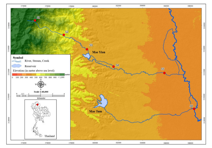
Lychee plantation areas are typically located at varying elevations on mountains to ensure proper drainage. This placement has direct effects on stream and river water flows and consequently influences pesticide residue, water quality and aquatic biodiversity. This research aims to examine the relationships between cypermethrin residue, water quality and phytoplankton diversity in the lychee plantation catchment area in Phayao Province, Thailand, from January to May 2022. The study area was divided into six sampling sites. Water samples were collected for the investigation of cypermethrin residual, physicochemical and biological water quality parameters. The water quality index was used as an overall measurement of water quality. The study also examined the diversity of phytoplankton species and the relationship among cypermethrin residue, water quality and phytoplankton diversity were studied using canonical correspondence analysis. The findings revealed an increasing trend of cypermethrin residue, with the maximum concentration reaching 29.43 mg/L in March. The trend of decreasing water quality scores from Station S1 to Station S5 indicated the influence of land use changes and human activities, especially in the community area (S5), which was characterized by deterioration of water quality. A total of 174 phytoplankton species were categorized into 5 divisions, with Chlorophyta accounting for 61.49% of the total, followed by Bacillariophyta (28.16%) and Cyanophyta (6.32%). The highest Shannon's diversity index and evenness were observed at Stations S3 and S4, respectively. The canonical correspondence analysis revealed an interesting relationship among cypermethrin residue, ammonia nitrogen, chlorophyll a and three algal species: Pediastrum simplex var. echinulatum, Pediastrum duplex var. duplex and Scenedesmus acutus at Station S3. This research implies that pesticide residue and water quality have a direct impact on phytoplankton distribution, illustrating the environmental challenges that occur in various geographical areas. This information can be applied to assist in the development of future sustainable land use management initiatives.

| [1] |
Székács A, Mörtl M, Darvas B (2015) Monitoring pesticide residues in surface and ground water in Hungary: Surveys in 1990–2015. Chemistry 1: 1–15. https://doi.org/10.1155/2015/717948 doi: 10.1155/2015/717948

|
| [2] | WHO (2022) Pesticide residues in food. Available from: https://www.who.int/news-room/fact-sheets/detail/pesticide-residues-in-food. |
| [3] | Shefali G, Kumar R, Sankhla MS, et al. (2021) Impact of pesticide toxicity in aquatic environment. Biointerface Res Appl Chem 11: 10131–10140. |
| [4] |
Stenström JR, Kreuger J, Goedkoop W (2021) Pesticide mixture toxicity to algae in agricultural streams – Field observations and laboratory studies with in situ samples and reconstituted water. Ecotoxicol Environ Saf 215: 112153. https://doi.org/10.1016/j.ecoenv.2021.112153 doi: 10.1016/j.ecoenv.2021.112153
|
| [5] |
Pimentel D (1955) Amounts of pesticides reaching target pests: Environmental impacts and ethics. J Agric Environ Ethics 8: 17–29. https://doi.org/10.1007/BF02286399 doi: 10.1007/BF02286399
|
| [6] |
Staley ZR, Harwood VJ, Rohr JR (2015) A synthesis of the effects of pesticides on microbial persistence in aquatic ecosystems. Crit Rev Toxicol 45: 813–836. https://doi.org/10.3109/10408444.2015.1065471 doi: 10.3109/10408444.2015.1065471
|
| [7] | Phayao Provincial Agriculture and Cooperatives Office (2020) Basic information Phayao province. Available from: https://www.opsmoac.go.th/phayao-dwl-preview-401391791843. |
| [8] | Phayao Provincial Agriculture and Cooperatives Office (2018) Lychee in Phayao 2018. Available from: https://www.opsmoac.go.th/phayao-dwl-preview-401391791843. |
| [9] |
Kuang L, Xu G, Tong Y, et al. (2022) Risk assessment of pesticide residues in Chinese litchis. J Food Prot 85: 98–103. https://doi.org/10.4315/JFP-21-268 doi: 10.4315/JFP-21-268
|
| [10] | Pongpinyo P, Jangbai S, Palkul W (2013) Pesticide residues analysis in lychee and longan fruits of Thailand. Available from: https://shorturl.asia/BMdHb. |
| [11] |
Sangchan W, Bannwarth M, Ingwersen J, et al. (2014) Monitoring and risk assessment of pesticides in a tropical river of an agricultural watershed in northern Thailand. Environ Monit Assess 186: 1083–1099. https://doi.org/10.1007/s10661-013-3440-8 doi: 10.1007/s10661-013-3440-8
|
| [12] | Lindsey R, Scott M (2010) What are phytoplankton. Available from: https://earthobservatory.nasa.gov/features/Phytoplankton. |
| [13] |
Munaron D, Mérigot B, Derolez V, et al. (2023) Evaluating pesticide mixture risks in French Mediterranean coastal lagoons waters. Sci Total Environ 867: 161303.https://doi.org/10.1016/j.scitotenv.2022.161303 doi: 10.1016/j.scitotenv.2022.161303
|
| [14] |
Wijewardene L, Wu N, Qu Y, et al. (2021) Influences of pesticides, nutrients, and local environmental variables on phytoplankton communities in lentic small water bodies in a German lowland agricultural area. Sci Total Environ 780: 146481. https://doi.org/10.1016/j.scitotenv.2021.146481 doi: 10.1016/j.scitotenv.2021.146481
|
| [15] |
Liu L, Zhu B, Wang GX (2015) Azoxystrobin-induced excessive reactive oxygen species (ROS) production and inhibition of photosynthesis in the unicellular green algae Chlorella vulgaris. Environ Sci Pollut Res Int 22: 7766–7775. https://doi.org/10.1007/s11356-015-4121-7 doi: 10.1007/s11356-015-4121-7
|
| [16] | Salman JM, Abdul-Adel E, AlKaim FA (2016) Effect of pesticide glyphosate on some biochemical features in Cyanophyta algae Oscillatoria limnetica. Int J Pharmtech Res 9: 355–365. |
| [17] |
Groner ML, Relyea RA (2011) A tale of two pesticides: how common insecticides affect aquatic communities. Freshw Biol 56: 2391–2404. https://doi.org/10.1111/j.1365-2427.2011.02667.x doi: 10.1111/j.1365-2427.2011.02667.x
|
| [18] |
Rumschlag SL, Mahon MB, Hoverman JT, et al. (2020) Consistent effects of pesticides on community structure and ecosystem function in freshwater systems. Nat Commun 11: 6333. https://doi.org/10.1038/s41467-020-20192-2 doi: 10.1038/s41467-020-20192-2
|
| [19] |
Rumschlag SL, Casamatta DA, Mahon MB, et al. (2022) Pesticides alter ecosystem respiration via phytoplankton abundance and community structure: Effects on the carbon cycle? Glob Chang Biol 28: 1091–1102. https://doi.org/10.1111/gcb.15952 doi: 10.1111/gcb.15952
|
| [20] |
Crossland NO, Shires SW, Bennett D (1982) Aquatic toxicology of cypermethrin. Ⅲ. Fate and biological effects of spray drift deposits in fresh water adjacent to agricultural land. Aquat Toxicol 2: 253–270. https://doi.org/10.1016/0166-445X(82)90015-7 doi: 10.1016/0166-445X(82)90015-7
|
| [21] |
Navarrete IA, Tee KAM, Unson JRS, et al. (2018) Organochlorine pesticide residues in surface water and groundwater along Pampanga River, Philippines. Environ Monit Assess 190: 289. https://doi.org/10.1007/s10661-018-6680-9 doi: 10.1007/s10661-018-6680-9
|
| [22] |
Kanyika-Mbewe C, Thole B, Makwinja R, et al. (2020) Monitoring of carbaryl and cypermethrin concentrations in water and soil in Southern Malawi. Environ Monit Assess 192: 595. https://doi.org/10.1007/s10661-020-08557-y doi: 10.1007/s10661-020-08557-y
|
| [23] |
Baruah P, Chaurasia N (2020) Ecotoxicological effects of alpha-cypermethrin on freshwater alga Chlorella sp.: Growth inhibition and oxidative stress studies. Environ Toxicol Pharmacol 76: 103347. https://doi.org/10.1016/j.etap.2020.103347 doi: 10.1016/j.etap.2020.103347
|
| [24] |
Yilmaz N, Yardimci CH, Elhag M, et al. (2018) Phytoplankton composition and water quality of Kamil Abduş lagoon (Tuzla Lake), Istanbul-Turkey. Water 10: 603. https://doi.org/10.3390/w10050603 doi: 10.3390/w10050603
|
| [25] |
Mihaylova VV, Todorov BR, Lyubomirova VV, et al. (2021) Determination of imidacloprid, cypermethrin and chlorpyrifos ethyl in water samples using high-performance liquid chromatography. Bulg Chem Commun 53: 55–60. https://doi.org/10.34049/bcc.53.1.5297 doi: 10.34049/bcc.53.1.5297
|
| [26] |
Hu W, Xie W, Chen S, et al. (2014) Separation of cis- and trans-Cypermethrin by reversed-phase high-performance liquid chromatography. J Chromatogr Sci 53: 612–618. https://doi.org/10.1093/chromsci/bmu094 doi: 10.1093/chromsci/bmu094
|
| [27] | APHA, AWWA, WEF (2017) Standard Methods for the Examination of Water and Wastewater, 23rd Ed., Washington: American Public Health Association. |
| [28] | Saijo Y (1975) A method for determination of chlorophyll. Jpn J Limnol 36: 103–109. |
| [29] |
Wintermans J, De Mots A. (1965) Spectrophotometric characteristics of chlorophylls a and b and their phenophytins in ethanol. Biochim Biophys Acta - Biophysics including Photosynthesis 109: 448–453. https://doi.org/10.1016/0926-6585(65)90170-6 doi: 10.1016/0926-6585(65)90170-6
|
| [30] | Pollution Control Department (2022) Water quality index: WQI. Available from: https://shorturl.asia/xhER6. |
| [31] | Shannon CE, Weaver W (1949) The mathematical theory of communication. Urbana: University of Illinois Press, 144. |
| [32] | Croasdale H, Flint EA (1986) Flora of New Zealand: freshwater algae, chlorophyta, desmids with ecological comments on their habitats. Wellington, New Zealand: V.R. Ward, Government Printer, 29–126. |
| [33] | Peerapornpisal Y (2015) Freshwater algae in Thailand. Chiang Mai: Chotanaprint, 440. |
| [34] | Wehr JD, Sheath RG (2003) Freshwater algae of north America. USA: Academic press. 772. |
| [35] |
Jayasiri M, Yadav S, Dayawansa NDK, et al. (2022) Spatio-temporal analysis of water quality for pesticides and other agricultural pollutants in Deduru Oya river basin of Sri Lanka. J Clean Prod 330: 129897. https://doi.org/10.1016/j.jclepro.2021.129897 doi: 10.1016/j.jclepro.2021.129897
|
| [36] |
Vryzas Z, Vassiliou G, Alexoudis C, et al. (2009) Spatial and temporal distribution of pesticide residues in surface waters in northeastern Greece. Water Res 43: 1–10. https://doi.org/10.1016/j.watres.2008.09.021 doi: 10.1016/j.watres.2008.09.021
|
| [37] | Thai Meteorological Department (2022) Thailand weather March 2022. Available from: https://shorturl.asia/TgsVp. |
| [38] |
Fijałkowska RK, Dragon K, Drożdżyński D, et al. (2022) Seasonal variation of pesticides in surface water and drinking water wells in the annual cycle in western Poland, and potential health risk assessment. Sci Rep 12: 3317. https://doi.org/10.1038/s41598-022-07385-z doi: 10.1038/s41598-022-07385-z
|
| [39] |
Sun X, Liu M, Meng J, et al. (2022) Residue level, occurrence characteristics and ecological risk of pesticides in typical farmland-river interlaced area of Baiyang lake upstream, China Sci Rep 12: 12049. https://doi.org/10.1038/s41598-022-16088-4 doi: 10.1038/s41598-022-16088-4
|
| [40] |
Gizińska J, Sojka M (2023) How climate change affects river and lake water temperature in central-west Poland; A case study of the Warta River catchment. Atmosphere 14: 330. https://doi.org/10.3390/atmos14020330 doi: 10.3390/atmos14020330
|
| [41] | U. S. EPA (2012) Conductivity. Available from: https://archive.epa.gov/water/archive/web/html/vms59.html. |
| [42] | U.S. Department of the Interior (2018) Turbidity and water. Available from: https://www.usgs.gov/special-topics/water-science-school/science/turbidity-and-water#overview. |
| [43] |
Zhong M, Liu S, Li K, et al. (2021) Modeling spatial patterns of dissolved oxygen and the impact mechanisms in a Cascade river. Front Environ Sci 9. https://doi.org/10.3389/fenvs.2021.781646 doi: 10.3389/fenvs.2021.781646
|
| [44] | Kumar R, Kumar A (2005) Water analysis | Biochemical oxygen demand, Encyclopedia of Analytical Science, 2 Eds., Elsevier, 315–324. https://doi.org/10.1016/B0-12-369397-7/00662-2 |
| [45] | U. S. EPA (2022) Indicators: Dissolved oxygen. Available from: https://www.epa.gov/national-aquatic-resource-surveys/indicators-dissolved-oxygen. |
| [46] |
Cui Z, Gao W, Li Y, et al. (2023) Dissolved oxygen and water temperature drive vertical spatiotemporal variation of phytoplankton community: Evidence from the largest diversion water source area. Int J Environ Res Public Health 20: 4307. https://doi.org/10.3390/ijerph20054307 doi: 10.3390/ijerph20054307
|
| [47] |
Liu L, Yang J, Lv H, Yu Z (2014) Synchronous dynamics and correlations between bacteria and phytoplankton in a subtropical drinking water reservoir, FEMS Microbiol Ecol 90: 126–138. https://doi.org/10.1111/1574-6941.12378 doi: 10.1111/1574-6941.12378
|
| [48] |
Verma N, Singh AK (2013) Development of biological oxygen demand biosensor for monitoring the fermentation industry effluent. ISRN Biotechnol 13: 1–6. https://doi.org/10.5402/2013/236062 doi: 10.5402/2013/236062
|
| [49] |
Susilowati S, Sutrisno J, Masykuri M, et al. (2018) Dynamics and factors that affects DO-BOD concentrations of Madiun river. AIP Conf Proc 2049: 020052. https://doi.org/10.1063/1.5082457 doi: 10.1063/1.5082457
|
| [50] | Bozorg-Haddad O, Delpasand M, Loáiciga HA (2021) 10 - Water quality, hygiene, and health. Economical, Political, and Social Issues in Water Resources, Elsevier, 217–257. https://doi.org/10.1016/B978-0-323-90567-1.00008-5 |
| [51] |
Ni W, Zhang J, Ding T, et al. (2012) Environmental factors regulating cyanobacteria dominance and microcystin production in a subtropical lake within the Taihu watershed, China. J Zhejiang Univ Sci 13: 311–322. https://doi.org/10.1631/jzus.A1100197 doi: 10.1631/jzus.A1100197
|
| [52] |
Li J, Glibert PM, Alexander JA, et al. (2012) Growth and competition of several harmful dinoflagellates under different nutrient and light conditions. Harmful Algae 13: 112–125. https://doi.org/10.1016/j.hal.2011.10.005 doi: 10.1016/j.hal.2011.10.005
|
| [53] | Tansamai S. Removal of orthophosphate and turbidity from municipal wastewater by polyaluminium chloride and water treatment sludge[master's thesis].[Bongkok]: Silpakorn University; 2022. 98 p. |
| [54] | Stubbs M (2016) Nutrients in agricultural production: A water quality overview. CRS 1: 1–38. |
| [55] |
Gu J, Yang J (2022) Nitrogen (N) transformation in paddy rice field: Its effect on N uptake and relation to improved N management. Crop Environ 1: 7–14. https://doi.org/10.1016/j.crope.2022.03.003 doi: 10.1016/j.crope.2022.03.003
|
| [56] | Hauck RD (1980) Mode of action of nitrification inhibitors. In Meisinger JJ, Randall GW, Vitosh ML. (eds.). Nitrification inhibitors-potentials and limitations, 19–32. https://doi.org/10.2134/asaspecpub38.c2 |
| [57] |
Sasakawa H, Yamamoto Y (1978) Comparison of the uptake of nitrate and ammonium by rice seedlings: influences of light, temperature, oxygen concentration, exogenous sucrose, and metabolic inhibitors. Plant Physiol 62: 665–669. https://doi.org/10.1104/pp.62.4.665 doi: 10.1104/pp.62.4.665
|
| [58] |
Yang HC, Kan CC, Hung TH, et al. (2017). Identification of early ammonium nitrate-responsive genes in rice roots. Sci Rep 7: 16885. https://doi.org/10.1038/s41598-017-17173-9 doi: 10.1038/s41598-017-17173-9
|
| [59] | Sirianuntapiboon S (2020) Domestic wastewater. IVEC Journal 4: 1–10. Available from https://so06.tci-thaijo.org/index.php/IVECJournal/article/view/242938 |
| [60] | Apirukmontri P, Duangmala K, Phewnil O, et al. (2021) Expansion of community size along riverbank and wastewater management for water quality in the Phetchaburi River. PHJBUU 16: 1–16 |
| [61] | Horn W (1992) The control of eutrophication of lakes and reservoirs. In Ryding SO, Rast W. (eds.). Man and the Biosphere Series Vol. 1. Paris: Unesco and The Parthenon Publishing Group 1989,314. https://doi.org/10.1002/iroh.19920770113 |
| [62] | Istvánovics V (2009) Eutrophication of lakes and reservoirs. In: Likens GE (editor), Encyclopedia of Inland Waters, Oxford: Elsevier, 157-65. |
| [63] | Khuantrairong T, Traichaiyaporn S (2008) Diversity and seasonal succession of the phytoplankton community in DoiTao Lake, Chiang Mai province, northern Thailand. Trop Nat Hist 8: 143–156. |
| [64] | U. S. EPA (2022) Climate change and harmful algal blooms. Available from: https://www.epa.gov/nutrientpollution/climate-change-and-harmful-algal-blooms. |
| [65] |
Su Y, Hu M, Wang Y (2022) Identifying key drivers of harmful algal blooms in a tributary of the three Gorges reservoir between different seasons: Causality based on data-driven methods. Environ Pollut 297: 118759. https://doi.org/10.1016/j.envpol.2021.118759 doi: 10.1016/j.envpol.2021.118759
|
| [66] |
Sidabutar T, Srimariana ES, Wouthuyzen S (2020) The potential role of eutrophication, tidal and climatic on the rise of algal bloom phenomenon in Jakarta bay. IOP Conf Series: Earth Environ Sci 429: 012021. https://doi.org/10.1088/1755-1315/429/1/012021 doi: 10.1088/1755-1315/429/1/012021
|
| [67] | Nkwuda N (2018) Water quality and phytoplankton as indicators of pollution in a tropical river. Conf Proc of 6th NSCB Biodiversity; Uniuyo 1: 83–89. |
| [68] |
Leelahakriengkrai P, Peerapornpisal Y (2010) Diversity of benthic diatoms and water quality of the Ping River, northern Thailand. Environment Asia 3: 82–94. https://doi.org/10.14456/ea.2010.12 doi: 10.14456/ea.2010.12
|
| [69] | Prasertsin T, Pekkoh J, Pathom-aree W, et al. (2014) Diversity, new and rare taxa of Pediastrum spp. in some freshwater resources in Thailand. Chiang Mai J Sci 41: 1065–1076. https://www.thaiscience.info/journals/Article/CMJS/10932953.pdf |
| [70] |
Phinyo K, Pekkoh J, Peerapornpisal Y (2017) Distribution and ecological habitat of Scenedesmus and related genera in some freshwater resources of northern and north-eastern Thailand. Biodiversitas 18: 1092–1099. https://doi.org/10.13057/biodiv/d180329 doi: 10.13057/biodiv/d180329
|
| [71] |
Peerapornpisal Y, Suphan S, Ngearnpat N, et al. (2008) Distribution of chlorophytic phytoplankton in northern Thailand. Biologia 63: 852–858. https://doi.org/10.2478/s11756-008-0112-1 doi: 10.2478/s11756-008-0112-1
|
| [72] |
Duangjan K, Wołowski K, Peerapornpisal Y (2014) New records of Phacus and Monomorphina taxa (euglenophyta) for Thailand. Pol Bot J 59: 235–247. https://doi.org/10.2478/pbj-2014-0039 doi: 10.2478/pbj-2014-0039
|
| [73] |
da Silva FJR, Lima FRS, do Vale DV, et al. (2013) High levels of total ammonia nitrogen as NH4+ are stressful and harmful to the growth of Nile tilapia juveniles. Acta Sci Biol Sci 35: 475-481. https://doi.org/10.4025/actascibiolsci.v35i4.17291 doi: 10.4025/actascibiolsci.v35i4.17291
|
| [74] |
Ding S, Chen M, Gong M, et al. (2018) Internal phosphorus loading from sediments causes seasonal nitrogen limitation for harmful algal blooms. Sci Total Environ 625: 872–84. https://doi.org/10.1016/j.etap.2020.103347 doi: 10.1016/j.etap.2020.103347
|
| [75] |
Nie J, Sun Y, Zhou Y (2020) Bioremediation of water containing pesticides by microalgae: mechanisms, methods, and prospects for future research. Sci Total Environ 707: 136080. https://doi.org/10.1016/j.scitotenv.2019.136080 doi: 10.1016/j.scitotenv.2019.136080
|
| [76] |
Morais MGD, Zaparoli M, Lucas BF, et al. (2022) Chapter 4 - microalgae for bioremediation of pesticides: overview, challenges, and future trends, Algal Biotechnology 63–78. https://doi.org/10.1016/B978-0-323-90476-6.00010-8 doi: 10.1016/B978-0-323-90476-6.00010-8
|
| [77] |
Noumssi B, Nguetsop VF, Théophile F, et al. (2021) Using diatom assemblages and physicochemical parameters to characterize waterfalls in Western highlands of Cameroun, West Africa. Asian J Environ Ecol 14: 21–33. https://doi.org/10.9734/ajee/2021/v14i230201 doi: 10.9734/ajee/2021/v14i230201
|
| [78] |
Dembowska EA (2021) The use of phytoplankton in the assessment of water quality in the lower section of Poland's largest river. Water 13: 3471. https://doi.org/10.3390/w13233471 doi: 10.3390/w13233471
|
| [79] |
Wu N, Faber C, Ulrich U, et al. (2018) Diatoms as an indicator for tile drainage flow in a German lowland catchment. Environ Sci Eur 30: 4. https://doi.org/10.1186/s12302-018-0133-5 doi: 10.1186/s12302-018-0133-5
|
| [80] |
Huang Y, Shen Y, Zhang S, et al (2022) Characteristics of phytoplankton community structure and indication to water quality in the lake in agricultural areas. Front Environ Sci 10: 1–14. https://doi.org/10.3389/fenvs.2022.833409 doi: 10.3389/fenvs.2022.833409
|
| [81] |
Huang Y, Xiao L, Li F, Xiao M, Lin D, Long X, Wu Z (2018) Microbial degradation of pesticide residues and an emphasis on the degradation of cypermethrin and 3-phenoxy benzoic acid: A review. Molecules 23: 2313. https://doi.org/10.3390/molecules23092313 doi: 10.3390/molecules23092313
|
| [82] |
Al-Mughrabi KI, Nazer IK, Al-Shuraiqi YT (1992) Effect of pH of water from the King Abdallah Canal in Jordan on the stability of cypermethrin. Crop Prot 11: 341–344. https://doi.org/10.1016/0261-2194(92)90060-I doi: 10.1016/0261-2194(92)90060-I
|


Figures(8) / Tables(1)

Jirapa Wongsa, Ramita Liamchang, Neti Ngearnpat, Kritchaya Issakul. Cypermethrin insecticide residue, water quality and phytoplankton diversity in the lychee plantation catchment area[J]. AIMS Environmental Science, 2023, 10(5): 609-627. doi: 10.3934/environsci.2023034


 DownLoad: