
Citation: M.A. Pardo, A.Riquelme1, J. Melgarejo. A tool for calculating energy audits in water pressurized networks[J]. AIMS Environmental Science, 2019, 6(2): 94-108. doi: 10.3934/environsci.2019.2.94
[1] | Laura Romero, Modesto Pérez-Sánchez, P. Amparo López-Jiménez . Improvement of sustainability indicators when traditional water management changes: a case study in Alicante (Spain). AIMS Environmental Science, 2017, 4(3): 502-522. doi: 10.3934/environsci.2017.3.502 |
[2] | Amir Hedayati Aghmashhadi, Giuseppe T. Cirella, Samaneh Zahedi, Azadeh Kazemi . Water resource policy support system of the Caspian Basin. AIMS Environmental Science, 2019, 6(4): 242-261. doi: 10.3934/environsci.2019.4.242 |
[3] | Chetan Dhokai, Ritesh Ramesh Palkar, Vicky Jain . Water saving in thermal power plant by use of membrane filter in cooling tower treatment. AIMS Environmental Science, 2022, 9(3): 282-292. doi: 10.3934/environsci.2022020 |
[4] | Bedassa D. Kitessa, Semu M. Ayalew, Geremew S. Gebrie, Solomon T. Teferi . Quantifying water-energy nexus for urban water systems: A case study of Addis Ababa city. AIMS Environmental Science, 2020, 7(6): 486-504. doi: 10.3934/environsci.2020031 |
[5] | Daniel Chuquin-Vasco, Geancarlo Torres-Yanacallo, Cristina Calderón-Tapia, Juan Chuquin-Vasco, Nelson Chuquin-Vasco, Ramiro Cepeda-Godoy . ANN for the prediction of isobutylene dimerization through catalytic distillation for a preliminary energy and environmental evaluation. AIMS Environmental Science, 2024, 11(2): 157-183. doi: 10.3934/environsci.2024009 |
[6] | Benjamin Hersh, Amin Mirkouei, John Sessions, Behnaz Rezaie, Yaqi You . A review and future directions on enhancing sustainability benefits across food-energy-water systems: the potential role of biochar-derived products. AIMS Environmental Science, 2019, 6(5): 379-416. doi: 10.3934/environsci.2019.5.379 |
[7] | Sonia Prestamburgo, Filippo Sgroi, Adriano Venudo, Carlo Zanin . Universal design as resilient urban space plan strategy. New scenarios for environmental resources' sustainable management. AIMS Environmental Science, 2021, 8(4): 321-340. doi: 10.3934/environsci.2021021 |
[8] | Arriya Mungsunti, Kevin A. Parton . The sustainability of the muang fai irrigation system of northern Thailand. AIMS Environmental Science, 2019, 6(2): 77-93. doi: 10.3934/environsci.2019.2.77 |
[9] | RAHMOUN Ibrahim, BENMAMAR Saâdia, RABEHI Mohamed . Comparison between different Intensities of Rainfall to identify overflow points in a combined sewer system using Storm Water Management Model. AIMS Environmental Science, 2022, 9(5): 573-592. doi: 10.3934/environsci.2022034 |
[10] | Misrak Girma, Abebayehu Assefa, Marta Molinas . Feasibility study of a solar photovoltaic water pumping system for rural Ethiopia. AIMS Environmental Science, 2015, 2(3): 697-717. doi: 10.3934/environsci.2015.3.697 |
Notation: Ai: Section of compensation tank i; ∆Hi(t): Pressure variation through the leak at node i; Ef(t): Friction energy for the simulation period; Einput(t):Input energy for the simulation period; EL(t): Energy through leaks for the simulation period; EN(t): Energy supplied by the reservoirs for the simulation period; EP(t): Energy supplied by pumping stations for the simulation period; EU(t):Energy supplied to users for the simulation period; hni(tk): piezometric head (m.w.c.) supplied from each of the water tanks at time tk; hi(tk): piezometric head (m.w.c.) at node i and time tk; n: Number of demand nodes of the network; np: Number of pumps; nn: number of reservoirs; m: Number of pipes of the network; Pi-ser: minimum service pressure required for supplied demand; qj(tk): Flow rate at line j at time interval tk; qni(tk): flow rate (m3 s-1) injected by the reservoir into the system; qli(tk): Leakage flow rate at node i at time interval tk; qlj(tk): Leakage flow rate at line j at time interval tk; qui(tk): flow rate delivered to users (m3 s-1); tk: Time interval; VL(t): Total leakage volume for the simulation period; Vinj(t): Total volume injected for the simulation period; VR (t): Total volume consumed by users for the simulation period; zi(tp): the levels of the free surface of water of tank i at the initial times; zi(t1): the levels of the free surface of water of tank i at the final times; α: Emitter exponent; γ : Specific weight of water; ∆Hi(t): Pressure variation through the leak; ∆EC(t): Total variation of the energy compensation of the tanks; Δtk: is the time interval (s).
Water and energy nexus in water pressurized networks (WPN) is probably one of the most relevant challenges that utility managers have to deal with around the world as managing water has been proved to be one of the biggest consumptive uses of energy and since only the adequate energy diagnosis entails the good efficient and energy sustainable management, a question also proposed in buildings [1,2] or museums [11]. In 2016, the International Energy Agency [19] stated that energy used in the water sector in 2014 is equivalent to 4% of global electricity consumption plus 50 million tons of oil equivalent of 2040.
The situation is similar in Europe, where the water sector is a major consumer of energy [20] and the energy consumption is equivalent to 3% of global electricity consumption [46]. In Spain, water sector consumed 5.8 % in 2008 [17], but these figures is explained as primary energy consumed in Spanish households are not included in this study.
In the water distribution step in the urban water cycle, energy use is within the ranges 0.1-0.6 kWh/m3 as stated by some approaches [8,9], and water losses flowing through breaks in pipelines are estimated as 12% in the United States, 24% in Europe [19], 30% in Spain and 8% in Alicante city [7]. Water losses represent one of the most difficult problems utility managers should address as an appropriate quality of service must be maintained (water should be delivered meeting pressure and quality requirements) while reducing water and energy consumption. Leakage produced in pipelines is calculated with regard to material, length and inlet pressure [15] and the water and energy relationship is also considered in WPN [12,13,14]. In order to reduce energy consumption in the distribution stage of the urban water cycle, some approaches have been proposed for the definition of performance indicators to assess practitioners and decision-makers [15,16], for pipeline rehabilitation [17,18], for the quantification of potential energy recovery [19,20] and the allocation of micro turbines[3].
In this context, the energy audit (with results in kWh) in WPNs [6] identifies the energy entering the system and also their end uses. This analysis shows that the energy balance is maintained —in other words, energy supplied by reservoir and pumps are equal to the sum of the energy consumed in taps and through leaks, energy dissipated in pipes and in valves and the energy stored or supplied by tanks—. With these calculations, the energy lost through leakage is quantified, and such energy loss results not only from the energy leaving the system through leaks (high figures depending on the energy footprint of water, e.g., desalinated water) but also the energy needed to overcome additional friction losses created by higher circulating flow rates through pipelines. Moreover, a performance assessment system that characterizes the network has been defined [5] to obtain valuable results to make right decisions in operation and management of water utilities. The use of models for the hydraulic simulation of WPN allowed practitioners to calculate flowrates and head losses in pipelines, demands and heads in nodes for the energy audit calculation. As WPN and District Metering Areas (DMA's) analysed can entail thousands of Km and consumption nodes, these formulas should not be manually but automatically computed (for high values of the calculation time).
The objective of this work is to propose a matlab-based educational software which allows practitioners to calculate the energy audits. This software is aimed for educational and professional purposes, as a tool useful to understand and calculate the energy audit losses in WPNs. The reader is encouraged to download the software package and source codes available at https://bit.ly/2FbNqdr. To ease the use, a graphical user interface (GUI) manages all the process guiding the users during the process and a video describing how to run the software has been released in youtube (in English and also in Spanish) (https://youtu.be/H59DgJKIbBQ). Some case studies in some municipalities [18,26] and in irrigation networks [25,26] have been performed with this software. This software is the first open-source software performing these calculations. Case A has been solved by civil engineers in University of Alicante and they tested this software after developing their own hand calculations. This experience has shown that UAEnergy allow students to move forward the learning process.
The work is organized as follows. Section 2 describes how to calculate the amount of energy used in WPN. UAEnergy software is described in section 3. Software requirements, input data required to run the model and the results are also commented herein. The cases studies analysed here are presented and discussed in section 4.
A calibrated hydraulic simulation model is required to solve the hydraulic problem. In order to perform the analysis in an extended period (tp, which can take values such as 1 year, 1 month, 1 day, etc.), it is necessary to divide duration time into ni intervals of time (Δtk; 5, 10, 15, 60 minutes, etc.). Thus, the total energy consumed in the extended period (tp = ni·Δtk) is obtained from the sum of the energies consumed in each time interval of the steady state simulation.
The external energy supplied by reservoirs is:
En(tp)=γ⋅tk=tp∑tk=0(nn∑i=1qni(tk)⋅hni(tk))⋅Δtk | (1) |
where γ is the specific weight of water, nn is the number of reservoirs, qni(tk) and hni(tk) are, respectively, the flow rate (m3 s-1) and piezometric head (m.w.c.) supplied from each of the water tanks at time tk, where Δtk is the time interval (s).This term represents the natural incoming energy into the system (in other words, the amount of energy which is available to supply water to the WPN).
The shaft work supplied by the pumps is:
Ep(tp)=γ⋅tk=tp∑tk=0(np∑i=1qpi(tk)⋅hpi(tk))⋅Δtk | (2) |
Where qpi(tk) and hpi(tk) are respectively the flow rate pumped by the station (m3 s-1) and the pump head (m.w.c.) at time tk. This calculation needs to be done for the np pumping stations that supply shaft work to the system at each discrete timetk. This energy is water energy and by considering the performance of each pumping unit (an essential parameter for energy optimisation) the electrical equivalent can be calculated. In this paper, and since the focus is on shaft work supplied by pumps and not energy consumed from electricity grids, these energy losses (pump efficiency and asynchronous motor efficiency) have not been included in the analysis. This term represents the incoming energy into the system required to satisfy water demand in consumption nodes. The water utility has to pay for this consumption of grid electicity (in other words, the energy operation costs in the WPN). The greater shaft work values, the more useful (and important) the energy audit will be (for the direct cost involved).
The energy delivered to users is:
Eu(tp)=γ⋅tk=tp∑tk=0(n∑i=1qui(tk)⋅hi(tk))⋅Δtk | (3) |
Where n is the number of demand nodes of the network, qui(tk) and hi(tk) are respectively the flow rate delivered to users (m3 s-1) and the piezometric head (m.w.c.) at node i and timetk. The energy delivered to users shows the efficiency of the use of the energy injected to the system (in an ideal WPN every energy input should convert into energy delivered to users).
Water losses are classified as background and bursts outflows (Lambert, 1994) and bursts are generally the natural evolution of background leakages generating changes of WPN hydraulic functioning, detectable as anomalies in monitored flow/pressure data. Since the location of background leakages is not known, it can be assumed that leakage is uniformly distributed along every pipeline of the water distribution system. Based on common modeling assumptions, water leakage at nodes is equal to the water losses produced in the half of all pipes connected to it and fully described in many approaches [27,28].
Leaks represent energy leaving the system, formally analogous to the energy delivered to users although from the point of view of the audit it is lost energy. This term is:
El(tp)=γ⋅tk=tp∑tk=0(n∑i=1qli(tk)⋅hi(tk))⋅Δtk | (4) |
With n being the number of nodes in the network, qli(tk) the leaked flow rate (m3 s-1) in the pipes adjacent to node i (and therefore associated with this node) at time tk, and hi(tk) is the piezometric head (m.w.c.) at time tk in the node where the leak qli(tk) has been concentrated. The energy lost through leaks are energy losses which have arisen in WPN because of the number of breaks along pipelines, being equal to zero in an ideal leak-free WPN.
The energy dissipated by friction is divided into energy dissipated in pipes and in control valves [25] to take into account the singularities of the headlosses originated by friction in pipes and also the influence of regulating valves (their influence is much lower in urban water networks than in irrigation networks).
The energy dissipated due to friction in pipes is:
Ef(tp)=γ⋅tk=tp∑tk=0(nl∑j=1qj(tk)⋅Δhj(tk))⋅Δtk | (5) |
where nl is the number of lines of the network, Δhj(tk) are friction losses (m.w.c.) in line j at time tk (this term is the difference in piezometric heads between the initial and final nodes), quj(tk) and qlj(tk) are, in line j, the flow rate necessary to satisfy the users demand and the flow rate that finally is lost through leaks, respectively. Therefore, the total flow rate in line j, qj(tk), is the sum of the two previous values. This term shows the hydraulic capacity of the network. A higher value indicates lower efficiency. Although this can be brought to values very close to zero, eliminating friction losses implies a very costly design. Target values depend on a balance between investment and running costs.
The energy dissipated in hydraulic valves is:
Ev(tp)=γ⋅tk=tp∑tk=0(nv∑j=1qvj(tk)⋅Δhvj(tk))⋅Δtk | (6) |
Where qv(tk) is the flow rate (m3 s-1) flowing through the hydraulic valve j at time tk, nv is the number of valves and Δhvj(tk) is the piezometric head (m.w.c.) lost in the hydraulic valve j (calculated as the difference between the upstream and downstream nodes of the valve). This term is also energy dissipated in WPN (this as a matter of pressure-flows regulation). Higher values may show potential energy savings using turbines (or pumps as turbines; PATs) for energy recovery.
Many WPN accumulate water during nights (low consumption) in a tank which release this amount of water during the day (peak consumption). If the simulation period is short (one or two days according to experience), the tanks can be considered mass and energy sources but if the simulation period is large, the contribution of this tank to the long-term analysis is zero.
The variation of potential energy stored in tanks is:
ΔEC(tp)=∑i=nCi=1(ECi(tp)−ECi(t1))=γ⋅∑i=nCi=1(Ai⋅(zi2(tp)−zi2(t1))/2) | (7) |
With Ai being the section of compensation tank i and zi(tp), zi(t1) the levels of the free surface of water of tank i at the initial and final times. The maximum variation of this energy, ΔECmax, obviously corresponds to total oscillation between empty and full tanks of the whole system.
From the preceding terms, where tp is the period of calculation of the expressions (commonly one day or one year), the following final balance results:
Einput(tp)=En(tp)+Ep(tp)=Eu(tp)+El(tp)+Ef(tp)+Ev(tp)+ΔEC(tp)==Eoutput(tp)+Edissipated(tp)+ΔEC(tp) | (8) |
Equation (8) states that the energy supplied by reservoirs and pumps to the water coming into the network is equal to the energy delivered to the users (throughout the water supplied) plus the losses (leakage and friction). From this balance, energy losses can be evaluated and efficient actions aimed to improve system's efficiency can be planned.
UAEnergy software is described in this section. Input data required to run the model—the software used here for solving the hydraulic problem in the WPN is Epanet [31] —, the internal process and the results are also commented herein
UAEnergy have three key requirements:
● A programming software like Matlab® running in the PC (its performance is similar on Windows®, Mac OS® X, and Linux®).
● Matlab® requires the user to choose a supported compiler installing a new compiler or selecting one of the multiple compilers installed in the personal computer.
● To have installed the Epanet programmer's toolkit, which is a dynamic link library (DLL) of functions that allows developers to customize Epanet computational engine for their own specific needs. The functions can be incorporated into 32-bit (and also into 64-bits) Windows applications written in C/C++, Delphi Pascal, Visual Basic, or any other language that can call functions within a windows DLL.
Some additional information for installing this has been released in the following link: https://personal.ua.es/en/mpardo/downloads/uaenergy/uaenergy.html. (In English and also in Spanish).
The key limitations of UAEnergy are that it requires to have the WPN modelled in Epanet (which may be a problem in some municipalities) and the user must know how to run Matlab® in his personal computer.
The input form data creates a GUI (Graphical User Interface) for the user to enter the model of the water pressurized network to send to the simulation program (Figure 1). The user can create the input file in two ways, by exporting the network through the application (Epanet) graphic interface or by writing directly in a notepad file (inserting the data in a specific order and separated by tabs). Once the input file (.inp extension) is created, no errors should appear when running this hydraulic simulation as any error in Epanet returns an error in UAEnergy. The most common errors in Epanet are missing data (in pipes, junctions, etc.), disconnected junctions/tanks/reservoirs, and negative pressures. The user has to check that when running the.inp model return successful hydraulic calculations.
The software consists of a variety of functions that apply the presented methodology. As it requires the application of a specific workflow, a GUI is programmed to guide the user through all the process (Figure 1). The button of the GUI is automatically activated after each step. Initially, the load button is active. The user can only press this button, which opens a menu to load the input file. Once the water network model is successfully loaded, 'Run' button is activated. There are not any additional input parameters that control the process.
The model loaded into UAEnergy has to consider the physical features of the WPN, which means data in nodes (base demands, elevation and hourly demand patterns), pipes (length, diameter, roughness, etc.), reservoirs (head), tanks (initial, minimum and maximum level of water, diameters, etc…), pumps (H-Q curves) and valves (type, settings, etc..) should be considered in the model. Moreover, the model has to be calibrated to represent real operation appropriately (which involves using observed flows/pressures in pipes/junctions). Without any doubt, the better the model represents real operation functioning, the more accurate the energy audit will be.
Leakage should be considered as pressure-dependent of node demands in the WPN model with the idea of adding an emitter—a device that models the flow through a nozzle— at each node of the network [18,28].
If the user wants to consider leakage in their WPN models, these emitters can be calibrated using an open source software called "UAleaks" which has also been developed and is available for downloading at: (http://bit.ly/2BmQjVP). A video describing the operation of this other software can be found at (http://bit.ly/2SvwF3O; [24]).
The outputs of the graphical user interface UAEnergy (Figure 2) are the water and energy audits shown in the graphical user interface in numbers, in graphs (Figure 2)
Moreover, a report file called "Name.inp – report.txt" and stored in the network path (this information is shown in the log menu shown Figure 1). This report file contains date of the simulation, the website where to download the software, the path where to find the model (whose energy audit has been calculated) and figures obtained for the water and energy audit. The user may import these figures in a spreadsheet for future analysis and also the graphs may be stored as an image in every format required (jpeg, tiff, pdf, etc…).
With the values of the water audit (which is calculated by UAEnergy as a consequence of the input hydraulic model considered), the student is allowed to check that the new model is taking into account the leakage flowrates, and the energy audit is shown to make the users understand that the outcoming water through leakage has a huge effect on energy losses.
The objective of the following case studies is to demonstrate the effectiveness of the proposed software in some water pressurized networks. Case A, B and C are synthetic networks to help students/users understand these concepts while case D, and E are real cases in urban areas (D is a district metering area in a Mediterranean city) and in irrigation networks (E represents the irrigation network in the University of Alicante).
This software has been used by every student of the course "Maintenance and operation of water distribution networks" and by some other MSc or Ph.D. students (in some other countries) who have known the existence of this software after some mailings and other advertises made by the software developers'. Although the key objective of this software it has been for students, some practitioners have shown their use in professional projects when managing WDNs. The explanation of these techniques involved two sessions (4 hours) to allow students to calculate the energy audit. The students informed about the good and quick results obtained in comparison with their hand calculation made and also commented that undertaking the audits in a real WDN would take a huge amount of time for a network such as a case A. In short, the students knew how to perform the calculation (and the high effort) manually.
Line | Initial Node | Final Node | Length (km) | Diameter (mm) | Node | Base demand (l/s) | Elevation (m) | Emitter Coeff. | Pattern |
10 | 9 | 21 | 2 | 300 | 11 | 5.8 | 5 | 0.006569 | 1 |
11 | 11 | 12 | 2 | 250 | 12 | 4 | 5 | 0.007507 | 1 |
12 | 12 | 13 | 2 | 250 | 13 | 2 | 3 | 0.006569 | 1 |
21 | 21 | 22 | 2 | 100 | 21 | 3 | 4 | 0.014076 | 1 |
22 | 22 | 23 | 2 | 100 | 22 | 2 | 8.5 | 0.013137 | 1 |
31 | 31 | 32 | 2 | 100 | 23 | 0 | 4 | 0.010322 | 1 |
111 | 11 | 21 | 4 | 150 | 31 | 1 | 2 | 0.005630 | 1 |
112 | 12 | 22 | 4 | 150 | 32 | 0 | 5 | 0.009853 | 1 |
113 | 13 | 23 | 4 | 150 | 33 | 0 | 2 | 0.006099 | 1 |
121 | 21 | 31 | 4 | 150 | Res | - | 1 | 2 | |
122 | 22 | 32 | 4 | 150 | |||||
123 | 23 | 33 | 4 | 150 | |||||
32 | 33 | 32 | 2.5 | 100 | |||||
1 | 22 | 11 | 1 | 100 | |||||
2 | 21 | 32 | 1 | 150 | |||||
3 | 23 | 32 | 1 | 100 | |||||
4 | 22 | 13 | 1 | 100 | |||||
Figure 3 shows the network layout and Table 1 shows the node and line data (number of nodes, n=9; number of lines, m=17). The values of the hourly coefficients, which consider water consumption at different hours of the day, are depicted in Table 2. Pipe roughness is 0.1 mm and the emitter exponent is α=1, 2 (corresponding to a mixed pipe-network [32,33]. |
Pattern1 | Time | 1 | 2 | 3 | 4 | 5 | 6 | 7 | 8 | 9 | 10 | 11 | 12 |
Coeff. | 0.6 | 0.5 | 0.45 | 0.45 | 0.5 | 0.6 | 0.7 | 1.1 | 1.3 | 1.2 | 1.1 | 1 | |
Time | 13 | 14 | 15 | 16 | 17 | 18 | 19 | 20 | 21 | 22 | 23 | 24 | |
Coeff. | 1.1 | 1.45 | 1.5 | 1.3 | 1.2 | 1.1 | 1.1 | 1.25 | 1.3 | 1.4 | 1 | 0.8 | |
Pattern 2 | Time | 1 | 2 | 3 | 4 | 5 | 6 | 7 | 8 | 9 | 10 | 11 | 12 |
Coeff. | 56.49 | 57.03 | 57.29 | 57.29 | 57.03 | 56.49 | 55.9 | 53.19 | 51.62 | 52.42 | 53.19 | 53.19 | |
Time | 13 | 14 | 15 | 16 | 17 | 18 | 19 | 20 | 21 | 22 | 23 | 24 | |
Coeff. | 50.36 | 49.92 | 51.62 | 52.42 | 53.19 | 53.19 | 52.03 | 51.62 | 50.79 | 53.92 | 55.28 | 56.49 |
In order to show this methodology can be used in some other networks, four additional cases are presented. Figure 4 shows the layout of networks B, C, D and E.
Case B (Figure 4) shows the network layout proposed for performing the very first energy audit calculations [6] while Case C is the anytown network (a very well-known hydraulic model used in many scientific works [34,35].
Case D shows a district metering area (DMA) in a western Mediterranean city of Spain [26] and it supplies water to 10000 inhabitants and consists of 561 nodes and 617 pipes, its total length is 10, 61 km. Finally, case E is the University of Alicante irrigation network [14]. The irrigation area of this garden has grown through time and new species have been added to the grass meadow (Festuca arundinacea, Pennisetum clandestinum and Poa annua), spread over an area of about 67 Ha. The network consists of 861 nodes, 891 pipes, a water well and four impeller pumps running in parallel and 160 electro valves upstream of the water discharge outlets, which are the hydrants. The total length of the network is 23 km.
As Case A is a synthetic WPN, each student had different level of leakage to calculate the energy audit. Table 3 shows the outputs obtained when the level of leakage is equal to 0.85 (it means that 15 % of the injected water into the WPN left the network through bursts). The computational time obtained was below 5 seconds. On the other hand, students have reached the same result but they informed that the calculation process was very time consuming (2 or 3 hours) and it made impossible to perform in usual District Metering Areas or WPNs (in which 1000 nodes and pipes are usual values) as this calculation time increases exponentially with regard to the number of nodes and lines.
UAEnergy | Student | |
Injected water (m3) | 3913.45 | 3913.45 |
Delivered water (m3) | 3326.40 | 3326.40 |
Real losses (m3) | 587.05 | 564.91 |
Volumetric error (%) | 0.000000 | 0.5657 |
Hydraulic Performance (%) | 84.9991 | 85.5649 |
En (kWh) | 568.47 | 568.48 |
Eu (kWh) | 352.10 | 352.10 |
El (kWh) | 71.42 | 71.41 |
Ef (kWh) | 144.95 | 144.94 |
Energetic error (%) | -0.0000 | 4.3361 10^-4 |
These results show the energy lost in water leaving the system through leakage and the comparison with some other models considering different levels of leakage show that the increase of water losses involves the increase of energy losses. If the network efficiency is 90 or 85%, the input energy is 536.29 kWh/day, which 352.10 kWh/day (61.94%) are delivered to final users, 71.42 kWh/day (12.57%) are lost through leakage and 144.95 kWh/day (25.49%) are dissipated in friction (Table 3).
Case B correspond to daily simulations for a synthetic leaky network. The hydraulic time step used to calculate the simulations is 1 minute for the simulation (Table 4). These values are exactly the same showed in [6] as the model corresponds to the daily simulation described there. This numbers can be obtained manually and they are showed here for the reader to be able to validate results.
B | C | D | E | |
En (kWh) | 386.65 | 306.44 | 282.94 | 590.48 |
Ep (kWh) | 977.75 | 8917.53 | 0 | 143.66 |
Eu (kWh) | 453.2 | 7068.18 | 253.90 | 701.94 |
El (kWh) | 232.67 | 0 | 28.11 | 0 |
Ef (kWh) | 549.8 | 1758.63 | 0.94 | 31.88 |
∆EC (kWh) | 128.51 | 367.98 | 0 | 0 |
Simulation period (h) | 24 | 24. | 48 | 72 |
Anytown (case C) includes two compensation tanks and three pumps working in parallel. The results showed that most of the energy input into the system (94.44%) is energy consumed by pumps while only 306.44 kWh/day is energy supplied by the reservoir. As this anytown network is not considering leakage and as it is also oversized, energy dissipated in pipes only represents 19.13% of the total amount of energy input into the WPN.
Case D intend to check the power of UAEnergy in real WPN supplying water to consumers. The UAEnergy user should identify these this WPN is oversized (Table 4; very low energy dissipated due to friction in pipes), a usual situation when operating WDN in urban areas. Results are obtained and the computational time is less than a minute when running the software and it seems to be impossible (or at least very time-consuming) to perform these hydraulic simulations in networks with so many pipes and nodes.
Case E represents the University of Alicante irrigation network where the energy is supplied by the reservoir (80.43%) and pumps (19.57%). These figures (Table 4) show that 4.38% of the input energy is dissipated by friction and the 95.62% left is delivered to crops.
This manuscript presents an open source engineering tool called UAEnergy. This software has been programmed with a general public license and an open source distribution to promote the download, use and share of the code and is available in a public repository. Practitioners are encouraged to undertake these calculations manually and to use UAenergy as a tool to validate results. Moreover, professional civil and hydraulic engineers also run this software with positive feedbacks, which means, in short, that they reached similar results with lower computational time.
Energy audits are calculated as the key result of this software. As the energy audit requires to have solved the hydraulic problem first, the water audit is also computed (not being the key result of this software) as water demands and leakages rates are required for the energy calculations. Five cases (two of them are real cases) have been performed and results highlight energy losses result not only from the energy leaving the system through leaks (which can be quite significant, e.g., desalinated water) but also the energy needed to overcome additional friction losses created by higher circulating flow rates through the pipes. Moreover, it also shows that these two real networks are oversized because of low values of energy dissipated through friction. It has also been pinpointed that this studies are relevant in WPN whose energy is consumed from electricity grids (Cases B, C and E).
The authors would like to acknowledge the valuable contributions of the editor and reviewers of this paper, as their comments and suggestions have helped to improve its contents. This work was supported by the research project "Desarrollo de herramientas especĺficas que permitan la gestión eficiente y sostenible del agua y de la energĺa en redes de agua a presión, GESAEN" through the 2016 call of the vicerrectorado de investigación, desarrollo e innovación de la universidad de Alicante GRE-16-08.
All authors declare no conflicts of interest in this paper.
[1] | Al-Ghamdi, A.S.(2011). Leakage–pressure relationship and leakage detection in intermittentwater distribution systems. J Water Supply ResTec. 60: 178–183. |
[2] |
Almandoz J, Cabrera E, ArreguiF, et al. (2005). Leakage Assessment through Water Distribution Network Simulation. J Water Res Pl-ASCE. 131:458–466. doi: 10.1061/(ASCE)0733-9496(2005)131:6(458)
![]() |
[3] | Bernardete C and António AC. (2018). Energy Recovery in Water Networks: Numerical DecisionSupport Tool for Optimal Site and Selection of Micro Turbines. J Water Res Pl-ASCE. 144: 04018004. Planningand Management |
[4] | Bijl DL, Bogaart PW, Kram T,et al. (2016). Long-term water demand for electricity, industry and households. EnvironSci Policy. 55: 75–86. |
[5] | Cabrera E, Gómez E, Cabrera JrE, et al. (2014). Energy assessment of pressurized water systems. J Water Res Pl-ASCE. 141: 4014095. |
[6] |
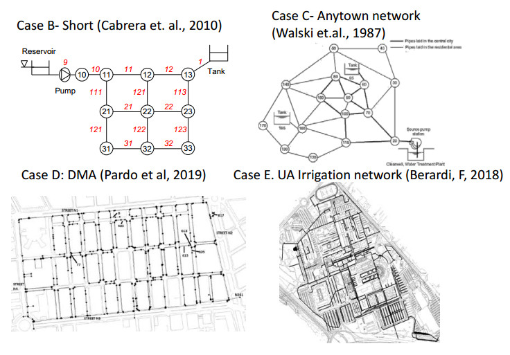
Cabrera E, Pardo MA, CobachoR, et al. (2010). Energy audit of water networks. J Water Res Pl-ASCE. 136:669-677. doi: 10.1061/(ASCE)WR.1943-5452.0000077
![]() |
[7] | Cantos JO, Rosique AC, delBusto IC, et al. (2018). RESILIENCIA EN EL CICLO URBANO DEL AGUA. EXTREMOS PLUVIOMÉTRICOS Y ADAPTACIÓN ALCAMBIO CLIMÁTICO EN EL ÁMBITO MEDITERRÁNEO. |
[8] | Cobacho R, Arregui F, SorianoJ, et al. (2014). Including leakage in network models: an application tocalibrate leak valves in EPANET. J Water Supply Res Tec. 64: 130–138. |
[9] | Comission CE. (2005). California'sWater – Energy Relationship. |
[10] | Dall'O G. (2011). GREENENERGY AUDIT-Manuale operativo per la diagnosi energetica e ambientale degliedifici. Edizioni Ambiente. |
[11] | EEO (1994). Introduction toEnergy Efficiency in Museums, Galleries, Libraries and Churches.. |
[12] |
Colombo AF, Karney BW. (2002) Energyand costs of leaky pipes: Toward comprehensive picture. J Water Res Pl-ASCE. 128: 441-450 doi: 10.1061/(ASCE)0733-9496(2002)128:6(441)
![]() |
[13] | Fernández García I, Creaco E,Rodríguez Díaz JA, et al. (2016). Rehabilitating pressurized irrigationnetworks for an increased energy efficiency. Agr WaterManage. 164: 212–222. |
[14] | Francesco Berardi (2018). Hydraulic anlysis and optimization of theirrigation network of the university of Alicante. Politecnico dibari i facoltà di ingegneria, Dicatech. |
[15] | Germanopoulos G. and Jowitt PW.(1989). LEAKAGE REDUCTION BY EXCESS PRESSURE MINIMIZATION IN A WATER SUPPLYNETWORK. P I Civil Eng 87: 195–214. |
[16] |
Greyvenstein B and van Zyl JE. (2007).An experimental investigation into the pressure - leakage relationship of somefailed water pipes. J Water Supply Res Tec. 56: 117–124. doi: 10.2166/aqua.2007.065
![]() |
[17] | Hardy L, Garrido A and Juana L.(2012). Evaluation of Spain's Water-Energy Nexus. Int J Water Resour D. 28: 151–170. |
[18] | Hernández E, Pardo MA, CabreraE, et al. (2010). Energy assessment of water networks: A casestudy. Water Distrib Syst Anal. 2010: 1168-1179. |
[19] | IEAIE (2016). Water EnergyNexus; Excerpt from the World Energy Outlook. |
[20] |
Larsen MAD and Drews M. (2019).Water use in electricity generation for water-energy nexus analyses: TheEuropean case. Sci Total Environ. 651: 2044–2058. doi: 10.1016/j.scitotenv.2018.10.045
![]() |
[21] | Lenzi C, Bragalli C, BolognesiA, et al. (2013). From energy balance to energy efficiency indicators includingwater losses. Water Sci and Technol. 13: 889–895. |
[22] |
Mamade A, Loureiro D, Alegre H,et al. (2017). A comprehensive and well tested energy balance for water supplysystems. Urban Water J. 14: 853–861. doi: 10.1080/1573062X.2017.1279189
![]() |
[23] | Murgui M, Cabrera E, Pardo MA,et al. (2009). Estimacióndel consumo de energía ligado al uso del agua en la ciudad de Valencia. Jornadasde Ingeniería del Agua. Madrid. |
[24] | Pardo M and Riquelme A. (2019). A software for considering leakage in waterpressurized networks. Comput Appl Eng Educ.2019: 1–13. |
[25] |
Pardo MA, Manzano J, Cabrera E,et al. (2013). Energy audit of irrigation networks. Biosyst Eng. 115: 89-101. doi: 10.1016/j.biosystemseng.2013.02.005
![]() |
[26] |
Pardo MA and Valdes-Abellan J. (2019).Pipe replacement by age only, how misleading could it be? Water Supp. 19:846–854. doi: 10.2166/ws.2018.131
![]() |
[27] | Pelli T and Hitz HU. (2000).Energy indicators and savings in water supply. JAm Water Works Ass.92: 55–62. |
[28] | Pérez-Sánchez M, Sánchez-RomeroF, Ramos H, et al. (2016). Modeling irrigation networks for the quantificationof potential energy recovering: A case study. Water. 8: 234. |
[29] | Picazo PM, Juárez J andGarcía-Márquez D. (2018). Energy consumption optimization in irrigationnetworks supplied by a standalone direct pumping photovoltaic system. Sustain. 10: 4203. |
[30] |
Farmani R, Walters GA, SavicDA. (2005). Trade-off between Total Cost and Reliability for Anytown WaterDistribution Network. JWater Res Pl-ASCE. 131: 161–171. doi: 10.1061/(ASCE)0733-9496(2005)131:3(161)
![]() |
[31] | Rossman LA. (2000). EPANET2: users manual. |
[32] | Telci I and Aral M. (2018).Optimal Energy Recovery from Water Distribution Systems Using Smart OperationScheduling. Water. 10: 1464. |
[33] | ValdesAbellan J, Pardo MA,TenzaAbril AJ. (2017). Observed precipitation trend changes in thewestern Mediterranean region. Int J Climatol.37: 1285-1296. |
[34] | Walski T. (2016). EnergyBalance for a Water Distribution System. World Environ and Water Resour Con 2016: 426–435. |
[35] |
Walski TM, Brill Jr ED, GesslerJ, et al. (1987). Battle of the network models: Epilogue. J Water Res Pl-ASCE. 113:191–203. doi: 10.1061/(ASCE)0733-9496(1987)113:2(191)
![]() |
Line | Initial Node | Final Node | Length (km) | Diameter (mm) | Node | Base demand (l/s) | Elevation (m) | Emitter Coeff. | Pattern |
10 | 9 | 21 | 2 | 300 | 11 | 5.8 | 5 | 0.006569 | 1 |
11 | 11 | 12 | 2 | 250 | 12 | 4 | 5 | 0.007507 | 1 |
12 | 12 | 13 | 2 | 250 | 13 | 2 | 3 | 0.006569 | 1 |
21 | 21 | 22 | 2 | 100 | 21 | 3 | 4 | 0.014076 | 1 |
22 | 22 | 23 | 2 | 100 | 22 | 2 | 8.5 | 0.013137 | 1 |
31 | 31 | 32 | 2 | 100 | 23 | 0 | 4 | 0.010322 | 1 |
111 | 11 | 21 | 4 | 150 | 31 | 1 | 2 | 0.005630 | 1 |
112 | 12 | 22 | 4 | 150 | 32 | 0 | 5 | 0.009853 | 1 |
113 | 13 | 23 | 4 | 150 | 33 | 0 | 2 | 0.006099 | 1 |
121 | 21 | 31 | 4 | 150 | Res | - | 1 | 2 | |
122 | 22 | 32 | 4 | 150 | |||||
123 | 23 | 33 | 4 | 150 | |||||
32 | 33 | 32 | 2.5 | 100 | |||||
1 | 22 | 11 | 1 | 100 | |||||
2 | 21 | 32 | 1 | 150 | |||||
3 | 23 | 32 | 1 | 100 | |||||
4 | 22 | 13 | 1 | 100 | |||||
Figure 3 shows the network layout and Table 1 shows the node and line data (number of nodes, n=9; number of lines, m=17). The values of the hourly coefficients, which consider water consumption at different hours of the day, are depicted in Table 2. Pipe roughness is 0.1 mm and the emitter exponent is α=1, 2 (corresponding to a mixed pipe-network [32,33]. |
Pattern1 | Time | 1 | 2 | 3 | 4 | 5 | 6 | 7 | 8 | 9 | 10 | 11 | 12 |
Coeff. | 0.6 | 0.5 | 0.45 | 0.45 | 0.5 | 0.6 | 0.7 | 1.1 | 1.3 | 1.2 | 1.1 | 1 | |
Time | 13 | 14 | 15 | 16 | 17 | 18 | 19 | 20 | 21 | 22 | 23 | 24 | |
Coeff. | 1.1 | 1.45 | 1.5 | 1.3 | 1.2 | 1.1 | 1.1 | 1.25 | 1.3 | 1.4 | 1 | 0.8 | |
Pattern 2 | Time | 1 | 2 | 3 | 4 | 5 | 6 | 7 | 8 | 9 | 10 | 11 | 12 |
Coeff. | 56.49 | 57.03 | 57.29 | 57.29 | 57.03 | 56.49 | 55.9 | 53.19 | 51.62 | 52.42 | 53.19 | 53.19 | |
Time | 13 | 14 | 15 | 16 | 17 | 18 | 19 | 20 | 21 | 22 | 23 | 24 | |
Coeff. | 50.36 | 49.92 | 51.62 | 52.42 | 53.19 | 53.19 | 52.03 | 51.62 | 50.79 | 53.92 | 55.28 | 56.49 |
UAEnergy | Student | |
Injected water (m3) | 3913.45 | 3913.45 |
Delivered water (m3) | 3326.40 | 3326.40 |
Real losses (m3) | 587.05 | 564.91 |
Volumetric error (%) | 0.000000 | 0.5657 |
Hydraulic Performance (%) | 84.9991 | 85.5649 |
En (kWh) | 568.47 | 568.48 |
Eu (kWh) | 352.10 | 352.10 |
El (kWh) | 71.42 | 71.41 |
Ef (kWh) | 144.95 | 144.94 |
Energetic error (%) | -0.0000 | 4.3361 10^-4 |
B | C | D | E | |
En (kWh) | 386.65 | 306.44 | 282.94 | 590.48 |
Ep (kWh) | 977.75 | 8917.53 | 0 | 143.66 |
Eu (kWh) | 453.2 | 7068.18 | 253.90 | 701.94 |
El (kWh) | 232.67 | 0 | 28.11 | 0 |
Ef (kWh) | 549.8 | 1758.63 | 0.94 | 31.88 |
∆EC (kWh) | 128.51 | 367.98 | 0 | 0 |
Simulation period (h) | 24 | 24. | 48 | 72 |