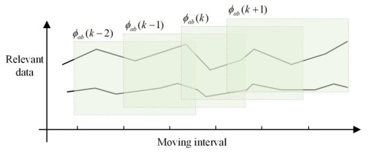
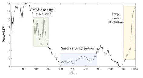
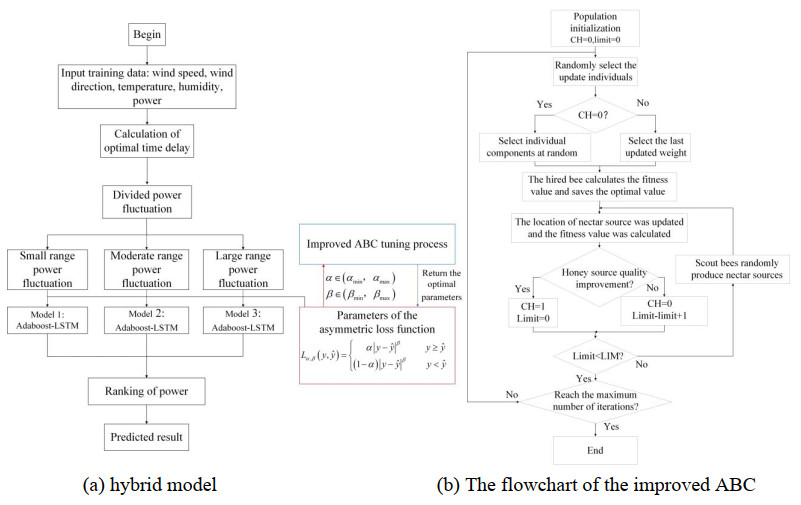
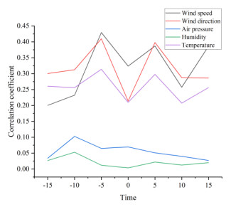
Wind energy, as a widely distributed, pollution-free energy, is strongly supported by the government. Accurate wind power forecasting technology ensures the balance of the power system and enhances the security of the system. In this paper, a wind power prediction model with the improved long short-term memory (LSTM) network and Adaboost algorithm was constructed based on the mismatch of data and power climb. This method was based on mutual information (MI) and power division (PD), named MI-PD-AdaBoost-LSTM. MI was used for quantifying the time delay between variables and power. Furthermore, to solve the relationship between wind speed and power in different weather fluctuation processes, the method of power fluctuation process division was proposed. Moreover, the asymmetric loss function of AdaBoost-LSTM was constructed to deal with the asymmetric characteristics of wind power. An improved artificial bee colony (ABC) algorithm, which overcame the local optimal problem, was used to optimize the asymmetric loss function parameters. Finally, the performance of different deep learning prediction models and the proposed prediction model was analyzed in the experiment. Numerical simulations showed that the proposed algorithm effectively improves the power prediction accuracy with different time scales and seasons. The designed model provides guidance for wind farm power prediction.
Citation: Feng Tian. A wind power prediction model with meteorological time delay and power characteristic[J]. AIMS Energy, 2025, 13(3): 517-539. doi: 10.3934/energy.2025020
Wind energy, as a widely distributed, pollution-free energy, is strongly supported by the government. Accurate wind power forecasting technology ensures the balance of the power system and enhances the security of the system. In this paper, a wind power prediction model with the improved long short-term memory (LSTM) network and Adaboost algorithm was constructed based on the mismatch of data and power climb. This method was based on mutual information (MI) and power division (PD), named MI-PD-AdaBoost-LSTM. MI was used for quantifying the time delay between variables and power. Furthermore, to solve the relationship between wind speed and power in different weather fluctuation processes, the method of power fluctuation process division was proposed. Moreover, the asymmetric loss function of AdaBoost-LSTM was constructed to deal with the asymmetric characteristics of wind power. An improved artificial bee colony (ABC) algorithm, which overcame the local optimal problem, was used to optimize the asymmetric loss function parameters. Finally, the performance of different deep learning prediction models and the proposed prediction model was analyzed in the experiment. Numerical simulations showed that the proposed algorithm effectively improves the power prediction accuracy with different time scales and seasons. The designed model provides guidance for wind farm power prediction.

| [1] |
Zhang Y, Kong X, Wang J, et al. (2024) Wind power forecasting system with data enhancement and algorithm improvement. Renewable Sustainable Energy Rev 196: 114349. https://doi.org/10.1016/j.rser.2024.114349 doi: 10.1016/j.rser.2024.114349

|
| [2] |
Tsai W, Hong C, Tu C, et al. (2023) A review of modern wind power generation forecasting technologies. Sustainability 15: 10757. https://doi.org/10.3390/su151410757 doi: 10.3390/su151410757
|
| [3] |
Hu Y, Liu H, Wu S, et al. (2024) Temporal collaborative attention for wind power forecasting. Appl Energy 357: 122502. https://doi.org/10.1016/j.apenergy.2023.122502 doi: 10.1016/j.apenergy.2023.122502
|
| [4] |
Tang Y, Yang K, Zhang S, et al. (2023) Wind power forecasting: A hybrid forecasting model and multi-task learning-based framework. Energy 278: 127864. https://doi.org/10.1016/j.energy.2023.127864 doi: 10.1016/j.energy.2023.127864
|
| [5] |
Huang Y, Liu GP, Hu W (2023) Priori-guided and data-driven hybrid model for wind power forecasting. ISA Trans 134: 380–395. https://doi.org/10.1016/j.isatra.2022.07.028 doi: 10.1016/j.isatra.2022.07.028
|
| [6] |
Nejati M, Amjady N, Zareipour H (2023) A new multi-resolution closed-loop wind power forecasting method. IEEE Trans Sustainable Energy 14: 2079–2091. https://doi.org/10.1109/TSTE.2023.3259939 doi: 10.1109/TSTE.2023.3259939
|
| [7] |
Wang Y, Zhao K, Hao Y, et al. (2024) Short-term wind power prediction using a novel model based on butterfly optimization algorithm-variational mode decomposition-long short-term memory. Appl Energy 366: 123313. https://doi.org/10.1016/j.apenergy.2024.123313 doi: 10.1016/j.apenergy.2024.123313
|
| [8] |
Heinrich R, Scholz C, Vogt S, et al. (2024) Targeted adversarial attacks on wind power forecasts. Mach Learn 113: 863–889. https://doi.org/10.1007/s10994-023-06396-9 doi: 10.1007/s10994-023-06396-9
|
| [9] |
Gu G, Li N, Pan Y, et al. (2024) Wind power forecasting based on a machine learning model: considering a coastal wind farm in Zhejiang as an example. Int J Green Energy 21: 2551–2558. https://doi.org/10.1080/15435075.2024.2319228 doi: 10.1080/15435075.2024.2319228
|
| [10] |
Liao CW, Wang I, Lin KP (2021) A fuzzy seasonal long short-term memory network for wind power forecasting. Mathematics 9: 71–86. https://doi.org/10.3390/math9111178 doi: 10.3390/math9111178
|
| [11] |
Lin Q, Cai H, Liu H, et al. (2024) A novel ultra-short-term wind power prediction model jointly driven by multiple algorithm optimization and adaptive selection. Energy 288: 129724. https://doi.org/10.1016/j.energy.2023.129724 doi: 10.1016/j.energy.2023.129724
|
| [12] |
He Y, Zhu C, Cao C (2024) A wind power ramp prediction method based on value-at-risk. Energy Convers Manage 315: 118767. https://doi.org/10.1016/j.enconman.2024.118767 doi: 10.1016/j.enconman.2024.118767
|
| [13] |
Wang C, Lin H, Hu H, et al. (2024) A hybrid model with combined feature selection based on optimized VMD and improved multi-objective coati optimization algorithm for short-term wind power prediction. Energy 293: 130684. https://doi.org/10.1016/j.energy.2024.130684 doi: 10.1016/j.energy.2024.130684
|
| [14] |
Sun B, Su M, He J (2024) Wind power prediction through acoustic data-driven online modeling and active wake control. Energy Convers Manage 319: 118920. https://doi.org/10.1016/j.enconman.2024.118920 doi: 10.1016/j.enconman.2024.118920
|
| [15] |
Safari N, Chung CY, Price G (2018) A novel multi-step short-term wind power prediction framework based on chaotic time series analysis and singular spectrum analysis. IEEE Trans Power Syst 33: 590–601. https://doi.org/10.1109/TPWRS.2017.2694705 doi: 10.1109/TPWRS.2017.2694705
|
| [16] |
Zhou B, Ma X, Luo Y (2019) Wind power prediction based on LSTM networks and nonparametric kernel density estimation. IEEE Access 7: 165279–165292. https://doi.org/10.1109/ACCESS.2019.2952555 doi: 10.1109/ACCESS.2019.2952555
|
| [17] |
Wang J, Qian Y, Zhang L, et al. (2024) A novel wind power forecasting system integrating time series refining, nonlinear multi-objective optimized deep learning and linear error correction. Energy Convers Manage 299: 117818. https://doi.org/10.1016/j.enconman.2023.117818 doi: 10.1016/j.enconman.2023.117818
|
| [18] |
Wang Y, Yang R, Sun L (2024) A novel structure adaptive discrete grey Bernoulli model and its application in renewable energy power generation prediction. Expert Syst Appl 255: 124481. https://doi.org/10.1016/j.eswa.2024.124481 doi: 10.1016/j.eswa.2024.124481
|
| [19] |
Zhou H, Wang X, Zhu R (2022) Feature selection based on mutual information with correlation coefficient. Appl Intell 52: 5457–5474. https://doi.org/10.1007/s10489-021-02524-x doi: 10.1007/s10489-021-02524-x
|
| [20] |
Belghit A, Lazri M, Ouallouche F, et al. (2023) Optimization of one versus All-SVM using AdaBoost algorithm for rainfall classification and estimation from multispectral MSG data. Adv Space Res 71: 946–963. https://doi.org/10.1016/j.asr.2022.08.075 doi: 10.1016/j.asr.2022.08.075
|
Figures(8) / Tables(10)

Feng Tian. A wind power prediction model with meteorological time delay and power characteristic[J]. AIMS Energy, 2025, 13(3): 517-539. doi: 10.3934/energy.2025020


 DownLoad: