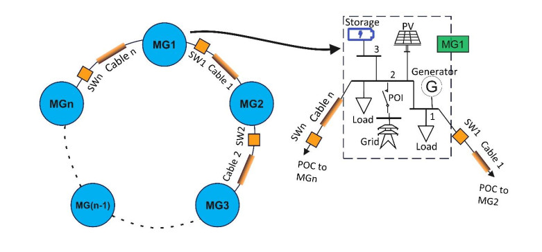
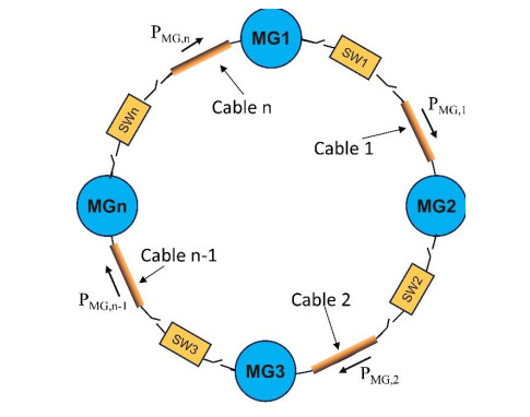
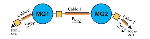
A ring-connected microgrid cluster can be formed by connecting geographically closed microgrids for mutual power sharing to increase the system's reliability. Real-time power balance within individual microgrids and power sharing among the microgrids of an islanded microgrid cluster would be challenging during contingencies if they are not properly sized and controlled. We propose a technique to design a ring-connected microgrid cluster that has several distributed energy resources. The amount of power flow via interconnecting cables was decided considering the size of the energy storage of the neighboring microgrids. A control system was designed to minimize the effect of severe transients in the neighboring microgrids in the network. The performance of the proposed technique was verified using a ring-connected microgrid cluster with four microgrids derived based on a real distribution system. The results illustrated that the proposed ring-connected microgrid cluster could maintain the power balance of the networked microgrid during the contingencies of neighboring microgrids, increasing the resiliency of the system compared to the radial and islanded operations.
Citation: W. E. P. Sampath Ediriweera, N. W. A. Lidula, R. Samarasinghe. Ring connected microgrid clusters for improved resiliency in distribution systems with high solar PV penetration[J]. AIMS Energy, 2024, 12(4): 872-904. doi: 10.3934/energy.2024041
A ring-connected microgrid cluster can be formed by connecting geographically closed microgrids for mutual power sharing to increase the system's reliability. Real-time power balance within individual microgrids and power sharing among the microgrids of an islanded microgrid cluster would be challenging during contingencies if they are not properly sized and controlled. We propose a technique to design a ring-connected microgrid cluster that has several distributed energy resources. The amount of power flow via interconnecting cables was decided considering the size of the energy storage of the neighboring microgrids. A control system was designed to minimize the effect of severe transients in the neighboring microgrids in the network. The performance of the proposed technique was verified using a ring-connected microgrid cluster with four microgrids derived based on a real distribution system. The results illustrated that the proposed ring-connected microgrid cluster could maintain the power balance of the networked microgrid during the contingencies of neighboring microgrids, increasing the resiliency of the system compared to the radial and islanded operations.

| [1] |
Xu Z, Yang P, Zheng C, et al. (2018) Analysis on the organization and development of multi-microgrids. Renewable Sustainable Energy Rev 81: 2204–2216. https://doi.org/10.1016/j.rser.2017.06.032 doi: 10.1016/j.rser.2017.06.032

|
| [2] |
Ediriweera WEPS, Lidula NWA (2022) Design and protection of microgrid clusters: A comprehensive review. AIMS Energy 10: 375–411. https://doi.org/10.3934/energy.2022020 doi: 10.3934/energy.2022020
|
| [3] |
Saleh MS, Althaibani A, Esa Y, et al. (2015) Impact of clustering microgrids on their stability and resilience during blackouts. 2015 International Conference on Smart Grid and Clean Energy Technologies (ICSGCE), 195–200. https://doi.org/10.1109/ICSGCE.2015.7454295 doi: 10.1109/ICSGCE.2015.7454295
|
| [4] |
Hossain MJ, Mahmud MA, Milano F, et al. (2015) Design of robust distributed control for interconnected microgrids. IEEE Trans Smart Grid 7: 2724–2735. https://doi.org/10.1109/TSG.2015.2502618 doi: 10.1109/TSG.2015.2502618
|
| [5] |
John T, Lam SP (2017) Voltage and frequency control during microgrid islanding in a multi-area multi-microgrid system. IET Gener Transm Dis 11: 1502–1512. https://doi.org/10.1049/iet-gtd.2016.1113 doi: 10.1049/iet-gtd.2016.1113
|
| [6] |
Liu T (2018) Energy management of cooperative microgrids: A distributed optimization approach. Int J Electr Power Energy Syst 96: 335–346. https://doi.org/10.1016/j.ijepes.2017.10.021 doi: 10.1016/j.ijepes.2017.10.021
|
| [7] |
Choobineh M, Silva-Ortiz D, Mohagheghi S (2018) An automation scheme for emergency operation of a multi-microgrid industrial park. IEEE Trans Ind Appl 54: 6450–6459. https://doi.org/10.1109/TIA.2018.2851210 doi: 10.1109/TIA.2018.2851210
|
| [8] |
Gregoratti D, Matamoros J (2015) Distributed energy trading: The multiple-microgrid case. IEEE Trans Ind Electron 62: 2551–2559. https://doi.org/10.1109/TIE.2014.2352592 doi: 10.1109/TIE.2014.2352592
|
| [9] |
Li Z, Shahidehpour M, Aminifar F, et al. (2017) Networked microgrids for enhancing the power system resilience. Proc IEEE 105: 1289–1310. https://doi.org/10.1109/JPROC.2017.2685558 doi: 10.1109/JPROC.2017.2685558
|
| [10] |
Wang Y, Rousis AO, Strbac G (2021) A three-level planning model for optimal sizing of networked microgrids considering a trade-off between resilience and cost. IEEE Trans Power Syst 36: 5657–5669. https://doi.org/10.1109/TPWRS.2021.3076128 doi: 10.1109/TPWRS.2021.3076128
|
| [11] |
Baghbanzadeh D, Salehi J, Gazijahani FS, et al. (2021) Resilience improvement of multi-microgrid distribution networks using distributed generation. Sustainable Energy Grids Netw 27: 100503. https://doi.org/10.1016/j.segan.2021.100503 doi: 10.1016/j.segan.2021.100503
|
| [12] |
Xie H, Teng X, Xu Y, et al. (2019) Optimal energy storage sizing for networked microgrids considering reliability and resilience. IEEE Access 7: 86336–86348. https://doi.org/10.1109/ACCESS.2019.2922994 doi: 10.1109/ACCESS.2019.2922994
|
| [13] |
Salehi N, Martínez-García H, Velasco-Quesada G (2022) Component sizing of an isolated networked hybrid microgrid based on operating reserve analysis. Energies 15: 17. https://doi.org/10.3390/en15176259 doi: 10.3390/en15176259
|
| [14] |
Wang Y, Rousis AO, Strbac G (2022) Resilience-driven optimal sizing and pre-positioning of mobile energy storage systems in decentralized networked microgrids. Appl Energy 305: 117921. https://doi.org/10.1016/j.apenergy.2021.117921 doi: 10.1016/j.apenergy.2021.117921
|
| [15] |
Lokesh V, Badar AQH (2023) Optimal sizing of res and bess in networked microgrids based on proportional peer-to-peer and peer-to-grid energy trading. Energy Storage 5: 464. https://doi.org/10.1002/est2.464 doi: 10.1002/est2.464
|
| [16] |
Ali L, Muyeen SM, Ghosh A, et al. (2020) Optimal sizing of networked microgrid using game theory considering the peer-to-peer energy trading. 2020 2nd International Conference on Smart Power and Internet Energy Systems (SPIES), 322–326. https://doi.org/10.1109/SPIES48661.2020.9243067 doi: 10.1109/SPIES48661.2020.9243067
|
| [17] |
Wang Z, Chen B, Wang J, et al. (2016) Networked microgrids for self-healing power systems. IEEE Trans Smart Grid 7: 310–319. https://doi.org/10.1109/TSG.2015.2427513 doi: 10.1109/TSG.2015.2427513
|
| [18] |
Chen C, Wang J, Ton D (2017) Modernizing distribution system restoration to achieve grid resiliency against extreme weather events: An integrated solution. Proc IEEE 105: 1267–1288. https://doi.org/10.1109/JPROC.2017.2684780 doi: 10.1109/JPROC.2017.2684780
|
| [19] |
Ali AY, Hussain A, Baek JW, et al. (2021) Optimal operation of networked microgrids for enhancing resilience using mobile electric vehicles. Energies 14: 142. https://doi.org/10.3390/en14010142 doi: 10.3390/en14010142
|
| [20] |
Wang Y, Rousis AO, Strbac G (2021) A resilience enhancement strategy for networked microgrids incorporating electricity and transport and utilizing a stochastic hierarchical control approach. Sustainable Energy Grids Netw 26: 100464. https://doi.org/10.1016/j.segan.2021.100464 doi: 10.1016/j.segan.2021.100464
|
| [21] |
Teimourzadeh S, Tor OB, Cebeci ME, et al. (2019) A three-stage approach for resilience-constrained scheduling of networked microgrids. J Mod Power Syst Clean Energy 7: 705–715. https://doi.org/10.1007/s40565-019-0555-0 doi: 10.1007/s40565-019-0555-0
|
| [22] |
Tostado-Vexliz M, Hasanien HM, Jordehi AR, et al. (2023) An interval-based privacy-aware optimization framework for electricity price setting in isolated microgrid clusters. Appl Energy 340: 121041. https://doi.org/10.1016/j.apenergy.2023.121041 doi: 10.1016/j.apenergy.2023.121041
|
| [23] |
Tostado-Vexliz M, Kamel S, Aymen F, et al. (2022) A stochastic-IGDT model for energy management in isolated microgrids considering failures and demand response. Appl Energy 317: 119162. https://doi.org/10.1016/j.apenergy.2022.119162 doi: 10.1016/j.apenergy.2022.119162
|
| [24] |
Tostado-Vexliz M, Hasanien HM, Jordehi AR, et al. (2023) Risk-averse optimal participation of a DR-intensive microgrid in competitive clusters considering response fatigue. Appl Energy 339: 120960. https://doi.org/10.1016/j.apenergy.2023.120960 doi: 10.1016/j.apenergy.2023.120960
|
| [25] |
Schneider KP, Radhakrishnan N, Tang Y, et al. (2019) Improving primary frequency response to support networked microgrid operations. IEEE Trans Power Syst 34: 659–667. https://doi.org/10.1109/TPWRS.2018.2859742 doi: 10.1109/TPWRS.2018.2859742
|
| [26] |
Miao Y, Hynan P, Jouanne AV, et al. (2019) Current li-ion battery technologies in electric vehicles and opportunities for advancements. Energies 12: 1074. https://doi.org/10.3390/en12061074 doi: 10.3390/en12061074
|
| [27] |
Mitali J, Dhinakaran S, Mohamad A (2022) Energy storage systems: A review. Energy Storage Sav 1: 166–216. https://doi.org/10.1016/j.enss.2022.07.002 doi: 10.1016/j.enss.2022.07.002
|
| [28] |
Tian H, Qin P, Li K, et al. (2020) A review of the state of health for lithium-ion batteries: Research status and suggestions. J Clean Prod 261: 120813. https://doi.org/10.1016/j.jclepro.2020.120813 doi: 10.1016/j.jclepro.2020.120813
|
| [29] |
Rezvanizaniani SM, Liu Z, Chen Y, et al. (2014) Review and recent advances in battery health monitoring and prognostics technologies for electric vehicle (ev) safety and mobility. J Power Sources 256: 110–124. https://doi.org/10.1016/j.jpowsour.2014.01.085 doi: 10.1016/j.jpowsour.2014.01.085
|
| [30] | Mit EV (2008) A guide to understanding battery specifications. Massachussetts Institute of Technology. Available from: http://web.mit.edu/evt/summary_battery_specifications.pdf. |
| [31] |
Ma S, Jiang M, Tao P, et al. (2018) Temperature effect and thermal impact in lithium-ion batteries: A review. Prog Nat Sci Mater Int 28: 653–666. https://doi.org/10.1016/j.pnsc.2018.11.002 doi: 10.1016/j.pnsc.2018.11.002
|
| [32] |
Jayasena KNC, Jayamaha DKJS, Lidula NWA, et al. (2019) SoC based multi-mode battery energy management system for dc microgrids. 2019 Moratuwa Engineering Research Conference (MERCon), 468–473. https://doi.org/10.1109/MERCon.2019.8818765 doi: 10.1109/MERCon.2019.8818765
|
| [33] |
Pogaku N, Prodanovic M, Green TC (2007) Modeling, analysis and testing of autonomous operation of an inverter-based microgrid. IEEE Trans Power Electron 22: 613–625. https://doi.org/10.1109/TPEL.2006.890003 doi: 10.1109/TPEL.2006.890003
|
| [34] |
Ediriweera WS, Lidula N, Herath HDB (2023) Robust microgrids for distribution systems with high solar photovoltaic penetration. Arch Electr Eng 72: 785–809. http://dx.doi.org/10.24425/aee.2023.146050 doi: 10.24425/aee.2023.146050
|
| [35] |
Guo X, Guo H (2011) Simulation and control strategy of a micro-turbine generation system for grid connected and islanding operations. Energy Proc 12: 368–376. https://doi.org/10.1016/j.egypro.2011.10.050 doi: 10.1016/j.egypro.2011.10.050
|
| [36] |
Shao W, Wu R, Ran L, et al. (2020) A power module for grid inverter with in-built short-circuit fault current capability. IEEE Trans Power Electron 35: 10567–10579. https://doi.org/10.1109/TPEL.2020.2978656 doi: 10.1109/TPEL.2020.2978656
|
| [37] |
Pan C, Tao S, Fan H, et al. (2021) Multi-objective optimization of a battery-supercapacitor hybrid energy storage system based on the concept of cyber-physical system. Electronics 10: 1801. https://doi.org/10.3390/electronics10151801 doi: 10.3390/electronics10151801
|
| [38] |
Naseri F, Farjah E, Allahbakhshi M, et al. (2017) Online condition monitoring and fault detection of large supercapacitor banks in electric vehicle applications. IET Electr Sys Transp 7: 318–326. https://doi.org/10.1049/iet-est.2017.0013 doi: 10.1049/iet-est.2017.0013
|
| [39] |
Yang H (2018) Estimation of supercapacitor charge capacity bounds considering charge redistribution. IEEE Trans Power Electron 33: 6980–6993. https://doi.org/10.1109/TPEL.2017.2764423 doi: 10.1109/TPEL.2017.2764423
|
| [40] | Kalbitz R, Puhane F (2022) Supercapacitor—A guide for the design-in process. Wurth Elektronik, Tech Rep. Available from: https://www.we-online.com/en/support/knowledge/application-notes?d = anp077-supercapacitor. |
| [41] | Qoria T, Cossart Q, Li C, et al. (2018) Wp3-control and operation of a grid with 100% converter-based devices. deliverable 3.2: Local control and simulation tools for large transmission systems. H2020 MIGRATE project. Available from: https://www.h2020-migrate.eu, 2018. |
| [42] |
Paquette AD, Divan DM (2015) Virtual impedance current limiting for inverters in microgrids with synchronous generators. IEEE Trans Ind Appl 51: 1630–1638. https://doi.org/10.1109/TIA.2014.2345877 doi: 10.1109/TIA.2014.2345877
|
| [43] |
Behabtu HA, Messagie M, Coosemans T, et al. (2020) A review of energy storage technologies' application potentials in renewable energy sources grid integration. Sustainability 12: 10511. https://doi.org/10.3390/su122410511 doi: 10.3390/su122410511
|
| [44] |
Georgious R, Refaat R, Garcia J, et al. (2021) Review on energy storage systems in microgrids. Electronics 10: 2134. https://doi.org/10.3390/electronics10172134 doi: 10.3390/electronics10172134
|
| [45] |
Wang H, Blaabjerg F (2014) Reliability of capacitors for dc-link applications in power electronic converters—An overview. IEEE Trans Ind Appl 50: 3569–3578. https://doi.org/10.1109/TIA.2014.2308357 doi: 10.1109/TIA.2014.2308357
|
| [46] |
Susanto J, Shahnia F, Ghosh A, et al. (2014) Interconnected microgrids via back-to-back converters for dynamic frequency support. 2014 Australasian Universities Power Engineering Conference (AUPEC), 1–6. https://doi.org/10.1109/AUPEC.2014.6966616 doi: 10.1109/AUPEC.2014.6966616
|
| [47] |
Worku MY, Hassan MA, Abido MA (2019) Real time energy management and control of renewable energy based microgrid in grid connected and island modes. Energies 12: 276. https://doi.org/10.3390/en12020276 doi: 10.3390/en12020276
|
| [48] |
Chakraborty S, Kramer B, Kroposki B (2009) A review of power electronics interfaces for distributed energy systems towards achieving low-cost modular design. Renewable Sustainable Energy Rev 13: 2323–2335. https://doi.org/10.1016/j.rser.2009.05.005 doi: 10.1016/j.rser.2009.05.005
|
| [49] |
Blaabjerg F, Chen Z, Kjaer S (2004) Power electronics as efficient interface in dispersed power generation systems. IEEE Trans Power Electron 19: 1184–1194. https://doi.org/10.1109/TPEL.2004.833453 doi: 10.1109/TPEL.2004.833453
|
| [50] |
Pawel S (2014) Matrix converter interfaces two three-phase AC systems as a component of smart-grid. 2014 International Symposium on Power Electronics, Electrical Drives, Automation and Motion, 683–688. https://doi.org/10.1109/SPEEDAM.2014.6872047 doi: 10.1109/SPEEDAM.2014.6872047
|
| [51] |
Carvalho EL, Blinov A, Chub A, et al. (2022) Grid integration of dc buildings: Standards, requirements and power converter topologies. IEEE Open J Power Electron 3: 798–823. https://doi.org/10.1109/OJPEL.2022.3217741 doi: 10.1109/OJPEL.2022.3217741
|
| [52] |
Yuan Y, Chang L, Song P (2007) A new front-end converter with extended hold-up time. 2007 Large Engineering Systems Conference on Power Engineering, 275–278. https://doi.org/10.1109/LESCPE.2007.4437392 doi: 10.1109/LESCPE.2007.4437392
|
| [53] | Electromagnetic compatibility part 4–11: Testing and measurement techniques voltage dips, short interruptions and voltage variations immunity tests. International Electrotechnical Commission, Geneva, Switzerland, Standard IEC 61000-4-11: 2020, 2020. Available from: https://webstore.iec.ch/publication/63503. |
| [54] | IEEE standard for the specification of microgrid controllers. IEEE, 1–43, 2018. https://doi.org/10.1109/IEEESTD.2018.8340204 |
| [55] | IEEE standard for interconnection and interoperability of distributed energy resources with associated electric power systems interfaces. IEEE Std 1547-2018 (Revision of IEEE Std 1547-2003), 1–138, 2018. https://doi.org/10.1109/IEEESTD.2018.8332112 |
| [56] | Anderson WW (2020) Resilience assessment of islanded renewable energy microgrids. Available from: https://apps.dtic.mil/sti/citations/AD1126753. |
| [57] |
Ediriweera WEPS, Lidula NWA (2023) Adaptive load shedding technique for energy management in networked microgrids. 2023 IEEE 17th International Conference on Industrial and Information Systems (ICIIS), 465–470. https://doi.org/10.1109/ICIIS58898.2023.10253509 doi: 10.1109/ICIIS58898.2023.10253509
|
| [58] |
Ediriweera WEPS, Lidula NWA (2023) Adaptive droop controller for energy management of islanded AC microgrids. 2023 Moratuwa Engineering Research Conference (MERCon), 292–297. http://dx.doi.org/10.1109/MERCon60487.2023.10355428 doi: 10.1109/MERCon60487.2023.10355428
|
Figures(17) / Tables(8)

W. E. P. Sampath Ediriweera, N. W. A. Lidula, R. Samarasinghe. Ring connected microgrid clusters for improved resiliency in distribution systems with high solar PV penetration[J]. AIMS Energy, 2024, 12(4): 872-904. doi: 10.3934/energy.2024041


 DownLoad: