Electric bus migration in Bengaluru with dynamic charging technologies

Ankit Kumar Begwani; Taha Selim Ustun; Ankit Kumar Begwani; Taha Selim Ustun

doi:10.3934/energy.2017.6.944

AIMS Energy

2017, Volume 5, Issue 6: 944-959. doi: 10.3934/energy.2017.6.944

Previous Article Next Article

Research article Topical Sections

Electric bus migration in Bengaluru with dynamic charging technologies

Ankit Kumar Begwani ¹,
Taha Selim Ustun ^{2
,
,}

1.
Department of Civil Engineering, PES Institute of Technology, Bangalore, India
2.
Electrical and Computer Engineering, Carnegie Mellon University, Pittsburgh, USA

Received: 13 October 2017 Accepted: 29 November 2017 Published: 06 December 2017

Rapid but unplanned urban development coupled with economic growth has resulted in congestion and pollution concerns in Indian cities. This forced India consider taking concrete steps towards design policies that would help stir the nation towards a more sustainable future. India, along with other bigger Asian economies like China, needs to address the growing global concerns over climate change and design their framework and policies to help cut down the greenhouse gas emissions. Transportation is a major source of pollution. A shift towards a pro-public transport policy would solve the traffic congestion problems and address the emission concerns. India has a significantly higher modal share of public transportation in its major cities. Public bus transport system acts as a lifeline to the India’s poor and middle class citizens. The following study focuses on the need for a replacement of conventional fossil fuel dependent buses with Electric buses in the existing public transport bus fleet in the city of Bengaluru. A design has been developed to utilize wireless charging technologies to realize electric bus migration in Bengaluru.

Keywords:

Citation: Ankit Kumar Begwani, Taha Selim Ustun. Electric bus migration in Bengaluru with dynamic charging technologies[J]. AIMS Energy, 2017, 5(6): 944-959. doi: 10.3934/energy.2017.6.944

Related Papers:

[1]	Alessandro Venditti, Claudio Frezza, Giacomo Rossi, Mirella Di Cecco, Giampiero Ciaschetti, Mauro Serafini, Armandodoriano Bianco . Secondary metabolites with ecologic and medicinal implications in Anthemis cretica subsp. petraea from Majella National Park. AIMS Molecular Science, 2016, 3(4): 648-660. doi: 10.3934/molsci.2016.4.648
[2]	Francisco Les, Zsuzsa Iffiú-Soltész, Josep Mercarder, Christian Carpéné . Tyramine activates lipid accumulation in rat adipocytes: influences of in vitro and in vivo administration. AIMS Molecular Science, 2017, 4(3): 339-351. doi: 10.3934/molsci.2017.3.339
[3]	Jin-Yih Low, Helen D. Nicholson . The up-stream regulation of polymerase-1 and transcript release factor(PTRF/Cavin-1) in prostate cancer: an epigenetic analysis. AIMS Molecular Science, 2016, 3(3): 466-478. doi: 10.3934/molsci.2016.3.466
[4]	Harkirat S. Sethi, Jessica L. Osier, Geordan L. Burks, Jennifer F. Lamar, Hana McFeeters, Robert L. McFeeters . Expedited isolation of natural product peptidyl-tRNA hydrolase inhibitors from a Pth1 affinity column. AIMS Molecular Science, 2017, 4(2): 175-184. doi: 10.3934/molsci.2017.2.175
[5]	Rachel L. Flores, Kayla Gonzales, Ryan W. Seaver, Brian T. Livingston . The skeletal proteome of the brittle star Ophiothrix spiculata identifies C-type lectins and other proteins conserved in echinoderm skeleton formation. AIMS Molecular Science, 2016, 3(3): 357-367. doi: 10.3934/molsci.2016.3.357
[6]	Charles A. Downs, Abdel A. Alli, Nicholle M. Johnson, My N. Helms . Cigarette smoke extract is a Nox agonist and regulates ENaC in alveolar type 2 cells. AIMS Molecular Science, 2016, 3(3): 439-453. doi: 10.3934/molsci.2016.3.439
[7]	Genu George, Sumita K. Chellappan, Mandagini Geetha, Padinjaradath S. Appukuttan . Possible molecular basis for macromolecular antigen attachment to host cells: their immune complex with plasma antibodies have unoccupied binding sites enabling binding to smaller ligands. AIMS Molecular Science, 2017, 4(1): 91-102. doi: 10.3934/molsci.2017.1.91
[8]	Sarika Amdekar, Avnish Kumar, Vinod Singh . Transcriptional activity of cytokines induced by oral administration of Lactobacillus casei and Lactobacillus acidophilus in experimental model of arthritis. AIMS Molecular Science, 2017, 4(2): 164-174. doi: 10.3934/molsci.2017.2.164
[9]	Noor Riyadh Thiab, Nicola King, Mary McMillan, Amer Almashhadany, Graham L Jones . Age-related protein and mRNA expression of glutathione peroxidases (GPx) and Hsp-70 in different regions of rat kidney with and without stressor. AIMS Molecular Science, 2016, 3(2): 125-137. doi: 10.3934/molsci.2016.2.125
[10]	Jin-Yih Low, Helen D. Nicholson . Investigating the role of caveolin-2 in prostate cancer cell line. AIMS Molecular Science, 2017, 4(1): 82-88. doi: 10.3934/molsci.2017.1.82

Abstract

1. Introduction

The following two-dimensional nonlinear multi-term time-fractional subdiffusion equations with initial and boundary conditions are considered in this paper:

$\begin{align} &D_{t}^{\boldsymbol{\alpha} }u = \Delta u+f(u),\ (x,y)\in \Omega,\ 0 < t\le T, \end{align}$

(1.1)

$\begin{align} &u(x,y,0) = g(x,y),\ (x,y)\in \Omega, \end{align}$

(1.2)

$\begin{align} &u(x,y,t) = 0,\ (x,y)\in \partial \Omega,\ 0\le t\le T, \end{align}$

(1.3)

where $\Omega = (0, L_1)\times (0, L_2)$ with the boundary $\partial \Omega$ , $f \; \in C^1(\mathbb{R})$ , and $g$ is a continuous function in $\Omega$ . The operator $D_{t}^{\boldsymbol{\alpha} }$ in (1.1) is defined by

$\begin{equation*} D_{t}^{\boldsymbol{\alpha} } = \sum\limits_{l = 1}^{J}{{{b}_{l}}D_{t}^{{{\alpha }_{l}}}},\ 0 < {{\alpha }_{J}} < {{\alpha }_{J-1}} < \cdots < {{\alpha }_{1}} < 1,\ and\ b_l > 0, \end{equation*}$

where $D_{t}^{{\alpha }_{l}}$ denotes the Caputo derivative with respect to $t$ , i.e.,

$\begin{equation*} D_{t}^{{{\alpha }_{l}}}u = \frac{1}{\Gamma (1-{{\alpha }_{l}})}\int_{0}^{t}{{{(t-s)}^{-{{\alpha }_{l}}}}\frac{\partial u(x,y,s)}{\partial s}ds}. \end{equation*}$

In order to describe the physical process better, some scholars use multi-term time fractional differential equations for modeling, such as the behavior of viscoelastic fluids^[1,2], the dispersion of pollutants^[3], and magnetic resonance imaging^[4]. The finite difference method^[5,6,7,8], the finite volume method ^[9,10], the fractional predictor-corrector method^[11], the finite element method^[12], the collocation method ^[13,14], and the spectral method^[15] have been developed for solving the multi-term time fractional equations. The work ^[16] proposed a fast linearized finite difference method for the nonlinear multi-term time-fractional wave equation using SOE approximation. Recently, a lot of work about the time fractional nonlinear subdiffusion equation has been published. For example, the paper ^[17] considered a Newton linearized Galerkin finite element method to solve the problem with non-smooth solutions in the time direction and provided an optimal error estimate by using the discrete fractional Gronwall-type inequality on the graded meshes. The paper ^[18] provided an efficient systematic framework for solving nonlinear fractional partial differential equations on unbounded domains and obtained an error estimate. Jiang et al. ^[19] proposed an efficient ADI scheme for the nonlinear subdiffusion equation with a weakly singular solution and obtained the pointwise-in-time error estimate. Li et al. ^[20] proposed a new tool, the refined discrete fractional-type Gr $\ddot{\text{o}}$ nwall inequality, which is used to derive a sharp pointwise-in-time error estimate of the L1 scheme for the problem. However, as far as the authors know, at present there is no work dedicated to the pointwise-in-time error estimate of the L1 scheme for the nonlinear multi-term time-fractional subdiffusion equation with weakly singular solutions. The present work is designed to fill this gap. Following ^[21,22], in the remainder of our paper, we make the following assumption:

Assumption 1.1. For all $(x, y, t)\in \bar{\Omega}\times (0, T]$ , we assume the solution satisfies

$\begin{align} \left| \frac{{{\partial }^{l}}u(x,y,t)}{\partial {{x}^{p}}\partial {{y}^{q}}} \right|\le C,\ l = 0,1,2,3,4,5,\ l = p+q, \end{align}$

(1.4)

$\begin{align} \left| \frac{{{\partial }^{k}}u(x,y,t)}{\partial {{t}^{k}}} \right|\le C(1+{{t}^{{{\alpha }_{1}}-k}}),\ k = 0,1,2, \end{align}$

(1.5)

where $C$ is a positive constant. $C$ in this paper represents a constant independent of time and space step, and $C$ in different positions represents different values.

This paper consists of the following sections. In Section 2, we construct a fully discrete scheme for the problem (1.1)–(1.3). In Section 3, some lemmas are introduced that will be used in the subsequent analysis. In Section 4, convergence and stability of the fully discrete scheme proposed in Section 2 are given, and we obtain the sharp pointwise-in-time error estimate. In Section 5, the theoretical analysis is verified by four numerical examples.

2. Fully discrete scheme

Let $M_1$ , $M_2$ , and $N$ be three positive integers. Divide space and time uniformly into $M_1 \times M_2$ and $N$ parts, respectively. Let $\{t_n|t_n = n\tau, \ 0\le n\le N\}$ be a uniform partition of $\left[0, T\right]$ with the time step $\tau = T/N$ . Let $h_1 = L_1/M_1$ and $h_2 = L_2/M_2$ be the spatial steps. So spatial grid points consist of $x_i = ih_1$ and $y_j = jh_2$ , where $i = 0, 1, \cdots, M_1$ and $j = 0, 1, \cdots, M_2$ . The spatial grid is represented by $\Omega' = \{(x_i, y_j)|i = 0, 1, \cdots, M_1, j = 0, 1, \cdots, M_2\}$ . Let $\Omega_h = \Omega'\cap\Omega$ , and $\partial\Omega_h = \Omega'\cap\partial\Omega$ . Defining $u_{i, j}^{n} = u(x_i, y_j, t_n)$ , the previous equations (1.1)–(1.3) at the grid point $\left(x_i, y_j, t_n\right)$ can be transformed into

$\begin{align} &D_{\tau }^{\boldsymbol{\alpha}}u_{i,j}^{n} = \delta _{x}^{2}u_{i,j}^{n}+\delta _{y}^{2}u_{i,j}^{n}+f(u_{i,j}^{n-1})+\sum\limits_{l = 1}^{J}{{{b}_{l}}({{r}_{l}})_{i,j}^{n}}+R_{i,j}^{n}+(\bar{r})_{i,j}^{n},\ (x_i,y_j)\in \Omega_h,\ 0 < t_n\le T, \end{align}$

(2.1)

$\begin{align} &u_{i,j}^0 = g(x_i,y_j),\ (x_i,y_j)\in \Omega_h, \end{align}$

(2.2)

$\begin{align} &u_{i,j}^n = 0,\ (x_i,y_j)\in \partial \Omega_h,\ 0\le t_n\le T, \end{align}$

(2.3)

where the notations in (2.1) will be given afterwards.

Applying an L1 formula for the multi-term time Caputo derivatives, i.e., set

$\begin{equation*} D_{\tau }^{\alpha_l }u_{i,j}^{n} = {{d}_{1}^{\alpha_l }}u_{i,j}^{n}-{{d}_{n}^{\alpha_l }}u_{i,j}^{0}-\sum\limits_{k = 1}^{n-1}{({{d}_{k}^{\alpha_l }}-{{d}_{k+1}^{\alpha_l }})u_{i,j}^{n-k}}, \end{equation*}$

where $d_{k}^{{{\alpha }_{l}}} = \frac{{{\tau }^{-{{\alpha }_{l}}}}[{{k}^{1-{{\alpha }_{l}}}}-{{(k-1)}^{1-{{\alpha }_{l}}}}]}{\Gamma (2-{{\alpha }_{l}})}$ . For simplicity, defining ${{d}_{k}} = \sum\limits_{l = 1}^{J}{{{b}_{l}}d_{k}^{{{\alpha }_{l}}}}$ , it yields that

$\begin{align} D_{\tau }^{\boldsymbol{\alpha} }u_{i,j}^{n}: = \sum\limits_{l = 1}^{J}{{b}_{l}}D_{\tau }^{\alpha_l }u_{i,j}^{n} = {{d}_{1}}u_{i,j}^{n}-{{d}_{n}}u_{i,j}^{0}-\sum\limits_{k = 1}^{n-1}{({{d}_{k}}-{{d}_{k+1}})u_{i,j}^{n-k}}. \end{align}$

(2.4)

A standard second-order approximation is used to discretize $\Delta u_{i, j}^n$ :

$\begin{equation*} \begin{split} &\Delta u_{i,j}^n \approx \delta _{x}^{2}u_{i,j}^{n}+\delta _{y}^{2}u_{i,j}^{n},\\ & \delta _{x}^{2}u_{i,j}^{n} = \frac{u_{i+1,j}^{n}-2u_{i,j}^{n}+u_{i-1,j}^{n}}{{{h}_{1}}^{2}},\\ &\delta _{y}^{2}u_{i,j}^{n} = \frac{u_{i,j+1}^{n}-2u_{i,j}^{n}+u_{i,j-1}^{n}}{{{h}_{2}}^{2}}. \end{split} \end{equation*}$

To approximate the nonlinear term $f(u_{i, j}^{n})$ , we utilize the backward formula, expressed as

$\begin{equation*} f(u_{i,j}^{n}) = f(u_{i,j}^{n-1})+(\bar{r})_{i,j}^{n}. \end{equation*}$

In (2.1), $({{r}_{l}})_{i, j}^{n}$ and $R_{i, j}^{n}$ are truncation errors, i.e.,

$\begin{equation*} \begin{split} &({{r}_{l}})_{i,j}^{n} = D_{\tau }^{{\alpha }_{l}}u_{i,j}^{n}-D_{t}^{{{\alpha }_{l}}}u_{i,j}^{n},\\ &R_{i,j}^{n} = \Delta u_{i,j}^n-(\delta _{x}^{2}u_{i,j}^{n}+\delta _{y}^{2}u_{i,j}^{n}). \end{split} \end{equation*}$

Leaving out the truncation errors in (2.1) and replacing $u_{i, j}^n$ by $U_{i, j}^n$ , the fully discrete scheme is obtained:

$\begin{align} &D_{\tau }^{\boldsymbol{\alpha} }U_{i,j}^{n} = \delta _{x}^{2}U_{i,j}^{n}+\delta _{y}^{2}U_{i,j}^{n}+f(U_{i,j}^{n-1}),\ (x_i,y_j)\in \Omega_h,\ 0 < t_n\le T, \end{align}$

(2.5)

$\begin{align} & U_{i,j}^{0} = g(x_i,y_j),\ (x_i,y_j)\in \Omega_h, \end{align}$

(2.6)

$\begin{align} & U_{i,j}^{n} = 0,\ (x_i,y_j)\in \partial \Omega_h,\ 0\le t_n\le T. \end{align}$

(2.7)

3. Preliminary lemmas

Lemma 3.1. For $(x_i, y_j)\in\Omega_h$ , $1\le n\le N$ , it holds that

$\begin{equation*} \left| (\bar{r})_{i,j}^{n} \right|\le C\tau t_n^{\alpha_1-1}. \end{equation*}$

Proof. Due to the continuity of $f'$ and the boundedness of $u$ , $f'(\zeta)$ is bounded, where $\zeta$ is between $u_{i, j}^{n}$ and $u_{i, j}^{n-1}$ . We obtain

$\begin{equation*} \left| (\bar{r})_{i,j}^{n} \right| = \left| f(u_{i,j}^{n})-f(u_{i,j}^{n-1}) \right|\le C\left| u_{i,j}^{n}-u_{i,j}^{n-1} \right| . \end{equation*}$

Then we estimate the truncation error in two cases (^[19], page 6). Note the condition (1.5).

Case A: $n\ge 2$

$\begin{equation*} \begin{split} \left| (\bar{r})_{i,j}^{n} \right|&\le C\left| u_{i,j}^{n}-u_{i,j}^{n-1} \right| \\ & = C\tau {{\left| \frac{\partial u(ih_1,jh_2,t)}{\partial t} \right|}_{t = \xi }}\ ({{t}_{n-1}} < \xi < {{t}_{n}})\\ & \le C\tau (1+{{\xi }^{{{\alpha }_{1}}-1}})\\ & \le C\tau (1+t_{n-1}^{{{\alpha }_{1}}-1}) \\ & \le C\tau (1+t_{n}^{{{\alpha }_{1}}-1}) \\ &\le C\tau t_{n}^{{{\alpha }_{1}}-1}, \end{split} \end{equation*}$

where we have used $t_{n-1}\simeq t_{n}$ for $n \geq 2$ in the penultimate inequality.

Case B: $n = 1$

$\begin{equation*} \begin{split} \left| (\bar{r})_{i,j}^{1} \right|&\le C\left| \int_{0}^{{{t}_{1}}}{\frac{\partial u(ih_1,jh_2,s)}{\partial s}ds} \right| \\ & \le C\int_{0}^{{{t}_{1}}}{\left| \frac{\partial u(ih_1,jh_2,s)}{\partial s} \right|ds} \\ & \le C\int_{0}^{{{t}_{1}}}{(1+{{s}^{{{\alpha }_{1}}-1}})ds} \\ & = C(\tau +\frac{1}{{{\alpha }_{1}}}{{\tau }^{{{\alpha }_{1}}}}) \\ & \le C{{\tau }^{{{\alpha }_{1}}}} = C\tau t_{1}^{{{\alpha }_{1}}-1}. \end{split} \end{equation*}$

The proof is completed. □

Lemma 3.2. For $(x_i, y_j)\in\Omega_h$ , $1\le n\le N$ , we have $\left|R_{i, j}^n\right|\le C(h_1^2+h_2^2)$ .

Proof. According to the Taylor expansion, we can see that

$\begin{equation*} \begin{split} \left|R_{i,j}^{n}\right|& = \left|\Delta u_{i,j}^n-(\delta _{x}^{2}u_{i,j}^{n}+\delta _{y}^{2}u_{i,j}^{n})\right|\\ & = \left|(u_{xx}(x_i,y_j,t_n)-\delta _{x}^{2}u_{i,j}^{n})+(u_{yy}(x_i,y_j,t_n)-\delta _{y}^{2}u_{i,j}^{n})\right|\\ &\le \frac{h_1^2}{12}\left| \left.\frac{{{\partial }^{4}}u(x,y_j,t_n)}{\partial {{x}^{4}}}\right|_{x = \xi_1}\right| +\frac{h_2^2}{12}\left| \left.\frac{{{\partial }^{4}}u(x_i,y,t_n)}{\partial {{y}^{4}}}\right|_{y = \xi_2}\right|\\ &\le C(h_1^2+h_2^2), \end{split} \end{equation*}$

where ${{x}_{i-1}} < \xi_1 < {{x}_{i+1}}$ , and ${{y}_{j-1}} < \xi_2 < {{y}_{j+1}}$ . □

Lemma 3.3. [, Lemma 6] $\left| \sum\limits_{l = 1}^{J}{{{b}_{l}}({{r}_{l}})_{i, j}^{n}} \right|\le C{{n}^{-\min \{2-{{\alpha }_{1}}, {{\alpha }_{1}}+1\}}}$ , for $(x_i, y_j)\in\Omega_h$ , $1\le n\le N$ .

Define the positive stability multipliers ${\theta }_{0} = \mu, \ {{\theta }_{n}} = \mu \sum\limits_{k = 1}^{n}{(d_k-d_{k+1}){{\theta }_{n-k}}}$ , where $\mu = d_{1}^{-1}$ .

Lemma 3.4. (^[24], Lemma 5.1) ${\theta }_{n}$ is a monotonically decreasing sequence with respect to $n$ . For $n = 0, 1, \cdots, N$ ,

$\begin{equation*} {{\theta }_{n}}\le b_{1}^{-1}\Gamma (2-{{\alpha }_{1}}){{\tau }^{{{\alpha }_{1}}}}{{(n+1)}^{{{\alpha }_{1}}-1}}. \end{equation*}$

Notation. $\theta _{n}$ here has the following relationship with $\sigma_n^{\boldsymbol{\alpha}}$ in Literature ^[24]: $\theta _{n} = \sigma_n^{\boldsymbol{\alpha}}$ .

Lemma 3.5. (^[24], Lemma 5.2, Corollary 5.1) For $n = 1, 2, \cdots, N,$

$\begin{equation*} \sum\limits_{j = 1}^{n}{{{j}^{-\beta }}{{\theta }_{n-j}}}\le b_{1}^{-1}\Gamma (2-{{\alpha }_{1}}){{\tau }^{{{\alpha }_{1}}}}[{{\kappa }_{\beta ,n}}{{(\frac{n}{2})}^{{{\alpha }_{1}}-1}}+\frac{1}{{{\alpha }_{1}}}{{(\frac{n}{2})}^{{{\alpha }_{1}}-\beta }}], \end{equation*}$

where $\beta\ge 0$ and

$\begin{equation*} {{\kappa }_{\beta ,n}} = \begin{cases} 1+\frac{1-{{n}^{1-\beta }}}{\beta -1},\ &\mathit{\text{ for }}\ \beta \ne 1, \\ 1+\ln n,\ &\mathit{\text{ for }}\ \beta = 1. \\ \end{cases} \end{equation*}$

If there exists $\underline{\alpha}$ , which satisfies $0 < \underline{\alpha} \leqslant \alpha_1 < 1$ , we have

$\begin{equation*} \sum\limits_{j = 1}^n j^{-\beta} \theta_{n-j} \leq \begin{cases}\hat{C} & \mathit{\text{ for }} \beta = 0, \\ \hat{C} K_{\beta, n} \tau t_n^{\alpha_1-1} & \mathit{\text{ for }} \beta > 1,\end{cases} \end{equation*}$

where constant $\hat{C}$ depends on $\underline{\alpha}$ and $T$ .

Lemma 3.6. (^[25], Lemma 5.1) If $\{y_n\}$ is a non-negative sequence, and it satisfies $y_n\le a_1t_n^{-\eta_1}+a_2t_n^{-\eta_2}+b\tau\sum\limits_{j = 1}^{n-1}{t_{n-j}^{\alpha-1}y_j}, \ 1\le n\le N$ , we get $y_n\le C(a_1t_n^{-\eta_1}+a_2t_n^{-\eta_2}), \ 1\le n\le N$ , where $0\le \eta_1, \eta_2 < 1$ , $a_1, a_2, b > 0$ , $0 < \alpha < 1$ and $N$ is a positive integer.

Suppose ${g^j}$ is an arbitrary mesh function; we define an integral operator $B_{t}^{\boldsymbol{\alpha} }$ , which satisfies $\ B_{t}^{\boldsymbol{\alpha} }({{g}^{0}}) = 0, \ B_{t}^{\boldsymbol{\alpha} }({{g}^{n}}) = \sum\limits_{j = 1}^{n}{{{\theta }_{n-j}}{{g}^{j}}}$ , for $n = 1, 2, \cdots, N$ .

Lemma 3.7. (^[23], Lemma 2) For any mesh function $\{U^j\}_{j = 0}^N$ , the following formula holds.

$\begin{equation*} B_{t}^{\boldsymbol{\alpha} }(D_{\tau }^{\boldsymbol{\alpha} }U^n) = U^n-U^0,\ for\ n = 1,2,\cdots,N. \end{equation*}$

4. Convergence and stability analysis

Theorem 4.1. If $U_{i, j}^n$ is the solution of (2.5)–(2.7) at point $(x_i, y_j, t_n)$ , and suppose $\left|U_{i_0, j_0}^{n}\right| = {{\left\| U^{n} \right\|}_{\infty }}$ , it holds that

$\begin{align} \left| U_{{{i}_{0}},{{j}_{0}}}^{n} \right|\le \left| U_{{{i}_{0}},{{j}_{0}}}^{0} \right|+ \sum\limits_{k = 1}^{n}{{{\theta }_{n-k}}\left| f(U_{{{i}_{0}},{{j}_{0}}}^{k-1}) \right|},\ for\ n\ge 0. \end{align}$

(4.1)

Proof. From (2.5), it is easy to see that $U_{i, j}^{n}$ satisfies

$\begin{align*} &(\sum\limits_{l = 1}^{J}{{{b}_{l}}d_{1}^{{{\alpha }_{l}}}}+\frac{2}{{h_1^{2}}}+\frac{2}{{h_2^{2}}})\left| U_{i,j}^{n} \right| \\ = &\left| \frac{U_{i+1,j}^{n}+U_{i-1,j}^{n}}{{h_1^{2}}}+\frac{U_{i,j+1}^{n}+U_{i,j-1}^{n}}{{h_2^{2}}}+\sum\limits_{l = 1}^{J}{\sum\limits_{k = 2}^{n}{{{b}_{l}}(d_{k-1}^{{{\alpha }_{l}}}-d_{k}^{{{\alpha }_{l}}})U_{i.j}^{n-k+1}}}+d_nU_{i,j}^0+f(U_{{i},{j}}^{n-1}) \right|. \end{align*}$

Based on (2.7) and the fact that $d_{k-1}^{\alpha_l} > d_k^{\alpha_l}$ , we have

$\begin{align*} &(\sum\limits_{l = 1}^{J}{{{b}_{l}}d_{1}^{{{\alpha }_{l}}}}+\frac{2}{{h_1^{2}}}+\frac{2}{{h_2^{2}}})\left| U_{i_0,j_0}^{n} \right| \\ \le & \left| \frac{2U_{{{i}_{0}},{{j}_{0}}}^{n}}{{h}_{1}^{2}} \right|+\left| \frac{2U_{{{i}_{0}},{{j}_{0}}}^{n}}{{h}_{2}^{2}} \right|+\sum\limits_{l = 1}^{J}{\sum\limits_{k = 2}^{n}{{{b}_{l}}(d_{k-1}^{{{\alpha }_{l}}}-d_{k}^{{{\alpha }_{l}}})\left| U_{{{i}_{0}},{{j}_{0}}}^{n-k+1} \right|}}+d_n\left|U_{i_0,j_0}^0\right|+\left| f(U_{{{i}_{0}},{{j}_{0}}}^{n-1}) \right|. \end{align*}$

Then, we obtain

$\begin{equation*} (\sum\limits_{l = 1}^{J}{{{b}_{l}}d_{1}^{{{\alpha }_{l}}}})\left| U_{i_0,j_0}^{n} \right|\le \sum\limits_{l = 1}^{J}{\sum\limits_{k = 2}^{n}{{{b}_{l}}(d_{k-1}^{{{\alpha }_{l}}}-d_{k}^{{{\alpha }_{l}}})\left| U_{{{i}_{0}},{{j}_{0}}}^{n-k+1} \right|}}+d_n\left|U_{i_0,j_0}^0\right|+\left| f(U_{{{i}_{0}},{{j}_{0}}}^{n-1}) \right|, \end{equation*}$

which, according to the definition of $D_{\tau }^{\boldsymbol{\alpha} }$ , is equivalent to the following expression:

$\begin{align} D_{\tau }^{\boldsymbol{\alpha}}\left| U_{i_0,j_0}^{n} \right|\le \left| f(U_{i_0,j_0}^{n-1}) \right|,\ 1\le n\le N. \end{align}$

(4.2)

By applying the integral operator to both sides of the above formula, we obtain

$\begin{equation*} B_{t}^{\boldsymbol{\alpha}}(D_{\tau }^{\boldsymbol{\alpha} }\left| U_{{{i}_{0}},{{j}_{0}}}^{n} \right|)\le B_{t}^{\boldsymbol{\alpha} }\left| f(U_{{{i}_{0}},{{j}_{0}}}^{n-1}) \right|. \end{equation*}$

Due to Lemma 3.7 and the above definition of $B_{t}^{\boldsymbol{\alpha} }$ , (4.1) holds for $n\ge 1$ . Obviously, (4.1) also holds for $n = 0$ . □

Theorem 4.2. Suppose that $u$ is the solution of (1.1)–(1.3) and satisfies Assumption 1.1, and that $U$ is the solution of (2.5)–(2.7). There exist positive constants $\tau_0$ and $h_0$ . When $\tau < \tau_0$ and $h_1, h_2 < h_0$ , it holds for $m > 0$ that

$\begin{align} {{\left\| {{u}^{m}}-{{U}^{m}} \right\|}_{\infty }}\le C(\tau t_{m}^{{\alpha }_{1}-1}+h_1^2+h_2^2). \end{align}$

(4.3)

Proof. For $m = 0$ , (4.3) holds obviously. Assuming that (4.3) holds for $m = 0, 1, 2\cdots n-1$ ( $n\ge 1$ ), then for sufficiently small $\tau$ , $h_1$ , $h_2$ , and $1\leq k \leq n$ , we obtain

$\begin{equation*} \begin{split} {{\left\| {{U}^{k-1}} \right\|}_{\infty }}&\le {{\left\| {{u}^{k-1}} \right\|}_{\infty }}+{{\left\| {{u}^{k-1}}-{{U}^{k-1}} \right\|}_{\infty }} \\ & \le \left\| {{u}^{k-1}} \right\|_{\infty }+1. \end{split} \end{equation*}$

Let us discuss whether the inequality (4.3) holds when $m = n$ . Let $e_{i, j}^m = u_{i, j}^m-U_{i, j}^m$ for $0\leq m\leq n$ . Subtracting (2.5)–(2.7) from (2.1)–(2.3), we obtain

$\begin{equation*} \begin{split} &D_{\tau }^{\boldsymbol{\alpha}}e_{i,j}^{m} = \delta _{x}^{2}e_{i,j}^{m}+\delta _{y}^{2}e_{i,j}^{m}+({{R}_{f}})_{i,j}^{m}+\sum\limits_{l = 1}^{J}{{{b}_{l}}({{r}_{l}})_{i,j}^{m}+R_{i,j}^{m}+(\bar{r})_{i,j}^{m}},\ (x_i,y_j)\in \Omega_h,\ 0 < t_m\le T, \\ & e_{i,j}^{0} = 0,\ (x_i,y_j)\in \Omega_h,\\ & e_{i,j}^{m} = 0,\ (x_i,y_j)\in \partial \Omega_h,\ 0\le t_m\le T, \end{split} \end{equation*}$

where $({{R}_{f}})_{i, j}^{m} = f(u_{i, j}^{m-1})-f(U_{i, j}^{m-1})$ . Considering the continuity of $f'$ , the boundedness of $u_{i, j}^{m-1}$ and $U_{i, j}^{m-1}$ , we have

$\begin{align} \left| ({{R}_{f}})_{i,j}^{m} \right| = \left| f(u_{i,j}^{m-1})-f(U_{i,j}^{m-1}) \right|\le C\left| e_{i,j}^{m-1} \right|. \end{align}$

(4.4)

Let $\left|e_{{{i}_{0}}, {{j}_{0}}}^{m}\right| = {{\left\| {{e}^{m}} \right\|}_{\infty }}$ . Using Lemmas 3.1–3.3 and inequality (4.4), similar to (4.2), it can be obtained that for $1\leq m\leq n$ ,

$\begin{align} D_{\tau }^{\boldsymbol{\alpha}}\left| e_{{{i}_{0},j_0}}^{m} \right|\le {{C}_{1}}\left| e_{{{i}_{0},j_0}}^{m-1} \right|+{{C}_{2}}{{m}^{-\min \{2-{{\alpha }_{1}},{{\alpha }_{1}}+1\}}}+{{C}_{3}}(h_1^2+h_2^2)+{{C}_{4}}\tau t_{m}^{{{\alpha }_{1}}-1}. \end{align}$

(4.5)

Applying the definition of $B_{t }^{\boldsymbol{\alpha}}$ again, and Lemmas 3.4 and 3.5, we can further obtain

$\begin{equation*} \begin{split} \left| e_{{{i}_{0},j_0}}^{m} \right|&\le C_1 \sum\limits_{k = 1}^{m}{{{\theta }_{m-k}}\left| e_{{{i}_{0},j_0}}^{k-1} \right|}+{{C}_{2}} \sum\limits_{k = 1}^{m}{{{\theta }_{m-k}}{{k}^{-\min \{2-{{\alpha }_{1}},1+{{\alpha }_{1}}\}}}}\\ &+C_3 \sum\limits_{k = 1}^{m}{{\theta }_{m-k}}{(h_1^2+h_2^2)}+{{C}_{4}}{{\tau }^{{{\alpha }_{1}}}} \sum\limits_{k = 1}^{m}{{{\theta }_{m-k}}{{k}^{{{\alpha }_{1}}-1}}} \\ & = {{C}_{1}} \sum\limits_{k = 1}^{m-1}{{{\theta }_{m-k-1}}\left| e_{{{i}_{0},j_0}}^{k} \right|}+{{C}_{2}} \sum\limits_{k = 1}^{m}{{{\theta }_{m-k}}{{k}^{-\min \{2-{{\alpha }_{1}},1+{{\alpha }_{1}}\}}}} \\ & +{{C}_{3}}\hat{C}(h_1^2+h_2^2)+{{C}_{4}}{{\tau }^{{{\alpha }_{1}}}} \sum\limits_{k = 1}^{m}{{{\theta }_{m-k}}{{k}^{{{\alpha }_{1}}-1}}} \\ & \le {{C}_{1}}b_{1}^{-1}\Gamma (2-{{\alpha }_{1}}){{\tau }^{{{\alpha }_{1}}}}\sum\limits_{k = 1}^{m-1}{{{(m-k)}^{{{\alpha }_{1}}-1}}\left| e_{{{i}_{0},j_0}}^{k} \right|} \\ & +{{C}_{2}}\hat{C}{{\kappa }_{{{\sigma }_{1}},m}}\tau t_{m}^{{{\alpha }_{1}}-1} +{{C}_{3}}\hat{C}(h_1^2+h_2^2) \\ & +{{C}_{4}}{{\tau }^{2{{\alpha }_{1}}}}b_{1}^{-1}\Gamma (2-{{\alpha }_{1}})\left[\left(1-\frac{1}{\alpha_1}\right)\left(\frac{m}{2}\right)^{\alpha_1-1}+\frac{m^{2\alpha_1-1}}{\alpha_12^{\alpha_1-1}}+\frac{1}{\alpha_1}\left(\frac{m}{2}\right)^{2\alpha_1-1}\right]\\ &\le C\left({{\tau }^{{{\alpha }_{1}}}}\sum\limits_{k = 1}^{m-1}{{{(m-k)}^{{{\alpha }_{1}}-1}}\left| e_{{{i}_{0},j_0}}^{k} \right|} +\tau t_{m}^{{{\alpha }_{1}}-1} +(h_1^2+h_2^2)\right), \end{split} \end{equation*}$

where $\sigma_1 = \min \{2-{{\alpha }_{1}}, {{\alpha }_{1}}+1\}$ . From Lemma 3.6, we have

$\begin{align} \left| e_{{{i}_{0},j_0}}^{m} \right| \le C(\tau t_{m}^{{{\alpha }_{1}}-1}+h_1^2+h_2^2),\ for\ 1\leq m\leq n. \end{align}$

(4.6)

In summary, the inequality (4.3) holds for $m = n$ , which finishes the mathematical induction. The proof is complete. □

Remark 4.1. The global maximum error of the numerical solution is

$\begin{equation*} \underset{1\le n\le N}{\mathop{\max\limits}}{{\left\| {{u}^{n}}-{{U}^{n}} \right\|}_{\infty }}\le C(\tau^{\alpha_1}+h_1^2+h_2^2). \end{equation*}$

When $t_n$ is away from 0, the local maximum error is

$\begin{equation*} {{\left\| {{u}^{n}}-{{U}^{n}} \right\|}_{\infty }}\le C(\tau+h_1^2+h_2^2). \end{equation*}$

Theorem 4.3. The fully discrete scheme (2.5)–(2.7) is stable with respect to the initial value. If $\hat{U}_{i, j}^n$ satisfies the following equations,

$\begin{align} & \sum\limits_{l = 1}^{J}{{{b}_{l}}D_{\tau }^{{{\alpha }_{l}}}\hat{U}_{i,j}^{n}} = \delta _{x}^{2}\hat{U}_{i,j}^{n}+\delta _{y}^{2}\hat{U}_{i,j}^{n}+f(\hat{U}_{i,j}^{n-1}),\ (x_i,y_j)\in \Omega_h,\ 0 < t_n\le T, \end{align}$

(4.7)

$\begin{align} & \hat{U}_{i,j}^{0} = \hat{g}(x_i,y_j),\ (x_i,y_j)\in \Omega_h, \end{align}$

(4.8)

$\begin{align} & \hat{U}_{i,j}^{n} = 0,\ (x_i,y_j)\in \partial \Omega_h,\ 0\le t_n\le T, \end{align}$

(4.9)

and ${{\left\| g- \hat{g}\right\|}_{\infty }}$ is sufficiently small, then

$\begin{align} {{\left\| \hat{e}^n \right\|}_{\infty }}\le C{{\left\| \hat{e}^0 \right\|}_{\infty }},\ for\ n\ge 0, \end{align}$

(4.10)

where $\hat{e}_{i, j}^n = U_{i, j}^n-\hat{U}_{i, j}^n$ .

Proof. Subtracting (4.7)–(4.9) from (2.5)–(2.7) and according to Theorem 4.1, we have

$\begin{equation*} \left| \hat{e}_{i_0,j_0}^n \right|\le \left| \hat{e}_{i_0,j_0}^0 \right|+ \sum\limits_{k = 1}^{n}{{{\theta }_{n-k}}\left| f(U_{i_0,j_0}^{k-1})-f(\hat{U}_{i_0,j_0}^{k-1}) \right|}, \end{equation*}$

where $\hat{e}_{i_0, j_0}^n = {{\left\| \hat{e}^n \right\|}_{\infty }}$ . (4.10) holds for $n = 0$ obviously. Suppose that (4.10) holds when $n = 0, 1, 2, \cdots, m-1(m\ge 1)$ , we have ${{\left\| \hat{U}^r \right\|}_{\infty }}\le {{\left\| \hat{e}^r \right\|}_{\infty }}+{{\left\| U^r \right\|}_{\infty }}\le C{{\left\| \hat{e}^0 \right\|}_{\infty }}+{{\left\| U^r \right\|}_{\infty }}\le 1+{{\left\| U^r \right\|}_{\infty }}$ on the condition that ${{\left\| \hat{e}^0 \right\|}_{\infty }}$ is small, for $r\le m-1$ . According to (4.3), $U_{i, j}^r$ is bounded. Then, combining the continuity of $f'$ and the boundedness of $\hat{U}_{i, j}^r$ , it holds that

$\begin{equation*} \begin{split} \left| \hat{e}_{i_0,j_0}^m \right|&\le \left| \hat{e}_{i_0,j_0}^0 \right|+ \sum\limits_{k = 1}^{m}{{{\theta }_{m-k}}\left| f(U_{i_0,j_0}^{k-1})-f(\hat{U}_{i_0,j_0}^{k-1}) \right|}\\ &\le \left| \hat{e}_{i_0,j_0}^0 \right|+C \sum\limits_{k = 1}^{m}{{{\theta }_{m-k}}\left| \hat{e}_{i_0,j_0}^{k-1} \right|}\\ &\le C\left| \hat{e}_{i_0,j_0}^0 \right|+C \sum\limits_{k = 1}^{m-1}{{{\theta }_{m-k-1}}\left| \hat{e}_{i_0,j_0}^{k} \right|}\\ &\le C\left| \hat{e}_{i_0,j_0}^0 \right|+C\tau \sum\limits_{k = 1}^{m-1}{t_{m-k}^{\alpha_1-1}\left| \hat{e}_{i_0,j_0}^{k} \right|}.\\ \end{split} \end{equation*}$

Due to Lemma 3.6, we have

$\begin{equation*} {{\left\| \hat{e}^m \right\|}_{\infty }}\le C{{\left\| \hat{e}^0 \right\|}_{\infty }}. \end{equation*}$

Therefore, the mathematical induction ends, and the proof is complete. □

5. Numerical experiments

Example 5.1. We first consider the following two-term time-fractional nonlinear subdiffusion equation with $b_1 = b_2 = 1$ .

$\begin{align} &D_{t}^{\alpha_1}u+D_{t}^{\alpha_2}u = \Delta u+u(1-u^2)+h(x,y,t),\ (x,y)\in \Omega,\ 0 < t\le T, \end{align}$

(5.1)

$\begin{align} &u(x,y,0) = g(x,y),\ (x,y)\in \Omega, \end{align}$

(5.2)

$\begin{align} &u(x,y,t) = 0,\ (x,y)\in \partial \Omega,\ 0\le t\le T, \end{align}$

(5.3)

where $h(x, y, t)$ and $g(x, y)$ are up to the exact solution. We set the exact solution to $t^{\alpha_1}sin(\pi x)sin(\pi y)$ , which satisfies Assumption 1.1. We consider the spatial domain $\Omega = (0, 1)\times (0, 1)$ and set $T = 1$ .

Above all, we compute the convergence order in spatial direction. We set $N = 1000$ so that the influence of errors in temporal direction can be ignored compared with errors in spatial direction. The maximum errors at $t_n = 1$ and rates, when $\alpha_1 = 0.4$ and $\alpha_2 = 0.3$ , are presented in . Numerical results show that the spatial accuracy is $O(h_1^2+h_2^2)$ . For studying temporal convergence rates, we define global errors $E_G$ and local errors $E_L$ by

$\begin{equation*} E_G = \underset{1\le n\le N}{\mathop{\max\limits}}{{\left\| U^n-u^n \right\|}_{\infty }},\ E_L = {{\left\| U^N-u^N \right\|}_{\infty }}. \end{equation*}$

Table 5.1. maximum errors at

$t_n = 1$ and spatial convergence rates for Example 5.1.

$M_1=M_2$	$4$	$8$	$16$	$32$	$64$
$E$	4.5780e-02	1.1335e-02	2.8363e-03	7.1957e-04	1.9089e-04
$rate$	2.0140	1.9987	1.9788	1.9144	*

| Show Table

DownLoad: CSV

Global errors and rates in show that the global temporal convergence order is $\alpha_1$ . When $t_n$ is far away from 0, results are shown in , and we get the local temporal accuracy $O(\tau)$ . All in all, numerical results are consistent with the theoretical analysis in Remark 1.

Table 5.2. global maximum errors and temporal convergence rates for Example 5.1.

$N=M_1^2=M_2^2$	$\alpha_1=0.3, \alpha_2=0.1$		$\alpha_1=0.5, \alpha_2=0.3$		$\alpha_1=0.7, \alpha_2=0.5$
$N=M_1^2=M_2^2$	$E_G$	$rate$	$E_G$	$rate$	$E_G$	$rate$
128	1.6333e-02	0.1690	1.0008e-02	0.3361	5.2012e-03	0.8184
256	1.4528e-02	0.1931	7.9278e-03	0.3660	2.9494e-03	0.6130
512	1.2708e-02	0.1926	6.1514e-03	0.3744	1.9284e-03	0.6260
1024	1.1120e-02	0.2038	4.7453e-03	0.4003	1.2496e-03	0.6518
2048	9.6547e-03	*	3.5956e-03	*	7.9532e-04	*

| Show Table

DownLoad: CSV

Table 5.3. local maximum errors at

$t_n = 1$ and temporal convergence rates for Example 5.1.

$N=M_1^2=M_2^2$	$\alpha_1=0.3, \alpha_2=0.1$		$\alpha_1=0.5, \alpha_2=0.3$		$\alpha_1=0.7, \alpha_2=0.5$
$N=M_1^2=M_2^2$	$E_L$	$rate$	$E_L$	$rate$	$E_L$	$rate$
128	5.0943e-03	0.8339	5.1615e-03	0.8359	5.2012e-03	0.8374
256	2.8579e-03	1.0536	2.8916e-03	1.0534	2.9109e-03	1.0531
512	1.3768e-03	0.9473	1.3933e-03	0.9477	1.4028e-03	0.9480
1024	7.1403e-04	1.0464	7.2235e-04	1.0460	7.2716e-04	1.0456
2048	3.4571e-04	*	3.4984e-04	*	3.5227e-04	*

| Show Table

DownLoad: CSV

Example 5.2. Secondly, we consider a two-dimensional three-term time-fractional nonlinear subdiffusion equation with $b_1 = b_2 = b_3 = 1$ .

$\begin{align} &D_{t}^{\alpha_1}u+D_{t}^{\alpha_2}u+D_{t}^{\alpha_3}u = \Delta u+u(1-u^2)+h(x,y,t),\ (x,y)\in \Omega,\ 0 < t\le T, \end{align}$

(5.4)

$\begin{align} &u(x,y,0) = g(x,y),\ (x,y)\in \Omega, \end{align}$

(5.5)

$\begin{align} &u(x,y,t) = 0,\ (x,y)\in \partial \Omega,\ 0\le t\le T, \end{align}$

(5.6)

where $\Omega = (0, 1)\times (0, 1)$ and $T = 1$ . We calculate $h(x, y, t)$ and $g(x, y)$ based on the exact solution

$\begin{equation*} t^{\alpha_1}sin(\pi x)sin(\pi y). \end{equation*}$

Numerical results are shown in Tables 5.4 and 5.5, which verify the theoretical analysis as well.

Table 5.4. global maximum errors and temporal convergence rates for Example 5.2.

$N=M_1^2=M_2^2$	$\alpha_1=0.3, \alpha_2=0.2, \alpha_3=0.1$		$\alpha_1=0.5, \alpha_2=0.4, \alpha_3=0.3$		$\alpha_1=0.7, \alpha_2=0.6, \alpha_2=0.5$
$N=M_1^2=M_2^2$	$E_G$	$rate$	$E_G$	$rate$	$E_G$	$rate$
128	1.7505e-02	0.1822	1.0842e-02	0.3657	4.9545e-03	0.7240
256	1.5428e-02	0.2052	8.4150e-03	0.3942	2.9994e-03	0.6375
512	1.3382e-02	0.2040	6.4030e-03	0.4000	1.9282e-03	0.6436
1024	1.1618e-02	0.2159	4.8524e-03	0.4227	1.2342e-03	0.6639
2048	1.0003e-02	*	3.6200e-03	*	7.7897e-04	*

| Show Table

DownLoad: CSV

Table 5.5. local maximum errors at

$t_n = 1$ and temporal convergence rates for Example 5.2.

$N=M_1^2=M_2^2$	$\alpha_1=0.3, \alpha_2=0.2, \alpha_3=0.1$		$\alpha_1=0.5, \alpha_2=0.4, \alpha_3=0.3$		$\alpha_1=0.7, \alpha_2=0.6, \alpha_2=0.5$
$N=M_1^2=M_2^2$	$E_L$	$rate$	$E_L$	$rate$	$E_L$	$rate$
128	4.8786e-03	0.8333	4.9371e-03	0.8351	4.9545e-03	0.8362
256	2.7380e-03	1.0534	2.7675e-03	1.0532	2.7751e-03	1.0529
512	1.3193e-03	0.9470	1.3337e-03	0.9474	1.3376e-03	0.9476
1024	6.8430e-04	1.0463	6.9158e-04	1.0460	6.9355e-04	1.0455
2048	3.3134e-04	*	3.3495e-04	*	3.3600e-04	*

| Show Table

DownLoad: CSV

Example 5.3. Thirdly, we investigate the scenario in which the nonlinear term is represented by $f(u) = sin(u)$ , which satisfies Lipschitz condition. The corresponding equation is formulated as follows:

$\begin{align} &D_{t}^{\alpha_1}u+D_{t}^{\alpha_2}u+D_{t}^{\alpha_3}u = \Delta u+sin(u)+h(x,y,t),\ (x,y)\in \Omega,\ 0 < t\le T, \end{align}$

(5.7)

$\begin{align} &u(x,y,0) = g(x,y),\ (x,y)\in \Omega, \end{align}$

(5.8)

$\begin{align} &u(x,y,t) = 0,\ (x,y)\in \partial \Omega,\ 0\le t\le T, \end{align}$

(5.9)

where $\Omega = (0, 1)\times (0, 1)$ and $T = 1$ . Similarly, we derive $h(x, y, t)$ and $g(x, y)$ based on the exact solution

$\begin{equation*} t^{\alpha_1}sin(\pi x)sin(\pi y). \end{equation*}$

The corresponding numerical results are presented in and . The global convergence order is $\alpha_1$ , and the local convergence order is 1 in the temporal direction.

Table 5.6. global maximum errors and temporal convergence rates for Example 5.3.

$N=M_1^2=M_2^2$	$\alpha_1=0.3, \alpha_2=0.2, \alpha_3=0.1$		$\alpha_1=0.5, \alpha_2=0.4, \alpha_3=0.3$		$\alpha_1=0.7, \alpha_2=0.6, \alpha_2=0.5$
$N=M_1^2=M_2^2$	$E_G$	$rate$	$E_G$	$rate$	$E_G$	$rate$
128	1.7753e-02	0.1908	1.0852e-02	0.3664	4.8924e-03	0.7058
256	1.5554e-02	0.2101	8.4178e-03	0.3945	2.9995e-03	0.6375
1024	1.1650e-02	0.2175	4.8527e-03	0.4227	1.2342e-03	0.6639
2048	1.0019e-02	*	3.6201e-03	*	7.7897e-04	*

| Show Table

DownLoad: CSV

Table 5.7. local maximum errors at

$t_n = 1$ and temporal convergence rates for Example 5.3.

$N=M_1^2=M_2^2$	$\alpha_1=0.3, \alpha_2=0.2, \alpha_3=0.1$		$\alpha_1=0.5, \alpha_2=0.4, \alpha_3=0.3$		$\alpha_1=0.7, \alpha_2=0.6, \alpha_2=0.5$
$N=M_1^2=M_2^2$	$E_L$	$rate$	$E_L$	$rate$	$E_L$	$rate$
128	5.0640e-03	0.8278	4.9983e-03	0.8256	4.8924e-03	0.8229
256	2.8530e-03	1.0552	2.8204e-03	1.0557	2.7656e-03	1.0561
512	1.3730e-03	0.9454	1.3568e-03	0.9449	1.3301e-03	0.9441
1024	7.1295e-04	1.0478	7.0484e-04	1.0484	6.9132e-04	1.0489
2048	3.4485e-04	*	3.4079e-04	*	3.3415e-04	*

| Show Table

DownLoad: CSV

Example 5.4. Finally, we consider a two-dimensional two-term time-fractional nonlinear subdiffusion equation with $b_1 = b_2 = 1$ , whose exact solution is unknown.

$\begin{align} &D_{t}^{\alpha_1}u+D_{t}^{\alpha_2}u = \Delta u+u(1-u),\ (x,y)\in \Omega,\ 0 < t\le T, \end{align}$

(5.10)

$\begin{align} &u(x,y,0) = \frac{1}{2}sin(\pi x)sin(\pi y),\ (x,y)\in \Omega, \end{align}$

(5.11)

$\begin{align} &u(x,y,t) = 0,\ (x,y)\in \partial \Omega,\ 0\le t\le T, \end{align}$

(5.12)

where $\Omega = (0, 1)\times (0, 1)$ and $T = 1$ .

The two-mesh method^[26] is applied to compute errors and convergence rates. We take $M_1 = M_2 = 60$ . $E_L$ is redefined by

$\begin{equation*} E_L = {{\left\| U^N-W^{2N} \right\|}_{\infty }}, \end{equation*}$

in which $W^n$ is the numerical solution of Example 5.4 with $\tau = T/2N$ . The local errors are shown in . The local temporal convergence rate $O(\tau)$ is consistent with Remark 1.

Table 5.8. local maximum errors at

$t_n = 1$ and temporal convergence rates for Example 5.4.

$N$	$\alpha_1=0.3, \alpha_2=0.1$		$\alpha_1=0.5, \alpha_2=0.3$		$\alpha_1=0.7, \alpha_2=0.5$
$N$	$E_L$	$rate$	$E_L$	$rate$	$E_L$	$rate$
32	6.8318e-05	1.0203	1.2027e-04	1.0285	1.4785e-04	1.0455
64	3.3682e-05	1.0103	5.8957e-05	1.0154	7.1633e-05	1.0270
128	1.6722e-05	1.0053	2.9166e-05	1.0086	3.5152e-05	1.0173
256	8.3302e-06	1.0027	1.4496e-05	1.0050	1.7367e-05	1.0117
512	4.1572e-06	*	7.2231e-06	*	8.6132e-06	*

| Show Table

DownLoad: CSV

Use of AI tools declaration

The authors declare they have not used Artificial Intelligence (AI) tools in the creation of this article.

Acknowledgments

The research is supported in part by the Natural Science Foundation of Shandong Province under Grant ZR2023MA077, Fundamental Research Funds for the Central Universities (No. 202264006), and the National Natural Science Foundation of China under Grant 11801026.

Conflict of interest

The authors declare there are no conflicts of interest.

References

[1]	International Energy Agency (2012) Understanding energy challenges in India. Policies, Players and Issues. IEEE Ind Appl Mag 17: 116.
[2]	Somalwar PRS, Apte MSM, Ikhe MYR (2014) A power sector of India by electric grid. IJRITCC 2: 774–777.
[3]	ICCT Fuels, International Council on Clean Transportation. Available from: http://www.theicct.org/.
[4]	M Release (2014) New transport scenarios for China, India, Latin America highlight role of cities in combatting climate change International Transport Forum at OECD releases projections for modal shares , emissions at Lima COP20 conference.
[5]	Ustun TS, Zayegh A, Ozansoy C (2013) Electric vehicle potential in Australia: its impact on smart grids. IEEE Ind Electron M 7: 15–25. doi: 10.1109/MIE.2013.2273947
[6]	Media Briefing Note, Centre for Science and Environment, Bengaluru, 2013. Available from: http://www.cseindia.org/userfiles/mbriefing_note.pdf.
[7]	EBSF: Designing the future of the bus, Press Kit, International Association of Public Transport. Available from: http://bit.ly/2z63wn4.
[8]	ZeEUS, Ebus Fact Sheet. Available from: http://bit.ly/2A20nVp.
[9]	ELIPTIC, Factor 100. Available from: http://bit.ly/2zHfsuU.
[10]	Wu Y, Zhang L (2017) Can the development of electric vehicles reduce the emission of air pollutants and greenhouse gases in developing countries? Transport Res D-Tre 51: 129–145. doi: 10.1016/j.trd.2016.12.007
[11]	Alessandrini A, Cignini F, Ortenzi F, et al. (2017) Advantages of retrofitting old electric buses and minibuses. Energ Procedia 126: 995–1002. doi: 10.1016/j.egypro.2017.08.260
[12]	Fok T, Prabhu A, Bachu P (2014) The high cost of low emissions standards for bus-based public transport operators in india: evidence from bangalore. Hepatology 16: 1322–1326.
[13]	Kenworthy J (2003) A study of 84 global cities, in transport energy use and greenhouse gases in Urban passenger transport systems. Available from: http://bit.ly/1kXoGZ4.
[14]	Asian Development Bank (2008) Managing Asian cities. ADB Publishing.
[15]	Krishna S (2013) A city in need of its citizens. The Hindu. Available from: http://bit.ly/1NTKtrn.
[16]	Centre for Science and Environment, Media briefing note. 2013. Available from: http://bit.ly/1TcOBqd.
[17]	Land Transport Authority Singapore (2011) Journeys: Sharing urban transport solutions.
[18]	Harish M (2012) A study on air pollution by automobiles in Bangalore city. Manage Res Pract 4: 25–36.
[19]	Midgley P (2009) Sharing urban transport solutions. Journeys-Sharing Urban Transport Solutions, 23–31.
[20]	Lajunen A (2014) Energy consumption and cost-benefit analysis of hybrid and electric city buses transp. Transport Res C-Emer 38: 1–15. doi: 10.1016/j.trc.2013.10.008
[21]	Banjac T, Trenc F, Katrašnik T (2009) Energy conversion efficiency of hybrid electric heavy-duty vehicles operating according to diverse drive cycles. Energ Convers Manage 50: 2865–2878. doi: 10.1016/j.enconman.2009.06.034
[22]	Ahluwalia R, Wang X, Kumar R (2012) Fuel Cell Transit Buses. Annual Report-IEA Advanced Fuel Cells. Available from: http://bit.ly/2zK1k0O.
[23]	Clark NN, Zhen F, Wayne WS, et al. (2007). Transit Bus Life Cycle Cost and Year 2007 Emissions Estimation. US DOT Federal Transit Administration. Carbon Dioxide, 2007.
[24]	Williamson R (2012) Transport for NSW Hybrid Bus Trial. Rare Consulting, Final Report.
[25]	BMTC in the red; city buses cannot go green, Bangalore Mirror. Available from: http://bit.ly/2An6z9Q.
[26]	Marvaniya RP, Gundaliya PJ (2014) Vehicular emission in Indian environment. IJFTET 4: 38–42.
[27]	BMTC Press Release. Available from: http://bit.ly/1Xmze55.
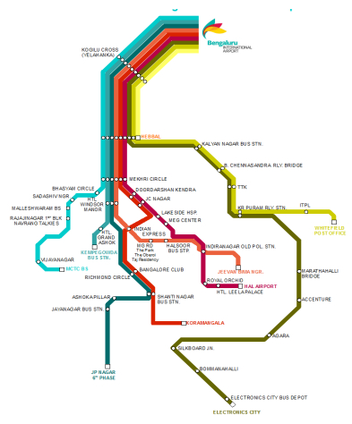
[28]	BMTC Bengaluru International Airport city bus shuttle route map. Available from: http://bit.ly/2A2Ujw3.
[29]	He X, Zhang S, Ke W, et al. (2017) Energy consumption and well-to-wheels air pollutant emissions of battery electric buses under complex operating conditions and implications on fleet electrification. J Clean Prod 171: 714–722.
[30]	Correa G, Muñoz P, Falaguerra T, et al. (2017) Performance comparison of conventional, hybrid, hydrogen and electric urban buses using well to wheel analysis. Energy 141: 537–549. doi: 10.1016/j.energy.2017.09.066
[31]	Sauer IL, Escobar JF, Silva MFPD, et al. (2015) Bolivia and paraguay: a beacon for sustainable electric mobility? Renew Sust Energ Rev 51: 910–925. doi: 10.1016/j.rser.2015.06.038
[32]	Teoh LE, Khoo HL, Goh SY, et al. (2017) Scenario-based electric bus operation: a case study of Putrajaya, Malaysia. International Journal of Transportation Science and Technology. Available from: http://www.sciencedirect.com/science/article/pii/S2046043017300540.
[33]	Wireless charging-the future for electric cars. Available from: http://www.bbc.com/news/technology-14183409.
[34]	Bombardier PRIMOVE Equipped E-buses start passenger service in Mannheim, Germany. Available from: http://bit.ly/1Xli3kd.
[35]	Review and Evaluation of wireless power transfer for Electric transit application (2014) FTA Research. Available from: http://1.usa.gov/1NTJSpA.
[36]	Wireless solar charging for electric buses. Available from: http://zd.net/1jnRQyO.
[37]	Volvo building an electric roadway to wirelessly charge buses. Available from: http://engt.co/2BGRuhq.
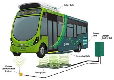
[38]	ARUP, World's most demanding electric bus route launched in Milton Keynes. Available from: http://bit.ly/2AJ63n0.
[39]	Miles J, Potter S (2014) Developing a viable electric bus service: the Milton Keynes demonstration project. Res Transp Econ 48: 357–363. doi: 10.1016/j.retrec.2014.09.063
[40]	Global Opportunities for SMEs in Electro-Mobility. Available from: http://bit.ly/2km56ut.
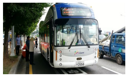
[41]	South Korean road wirelessly recharges OLEV buses, BBC News. Available from: http://bbc.in/1NzJwKs.
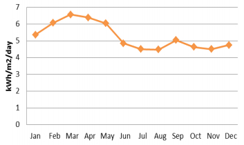
[42]	Solar Irradiation in Bengaluru, Karnataka, India. Available from: http://bit.ly/2iI5we5.

Reader Comments

Your name:*

Email:*
© 2017 the Author(s), licensee AIMS Press. This is an open access article distributed under the terms of the Creative Commons Attribution License (http://creativecommons.org/licenses/by/4.0)