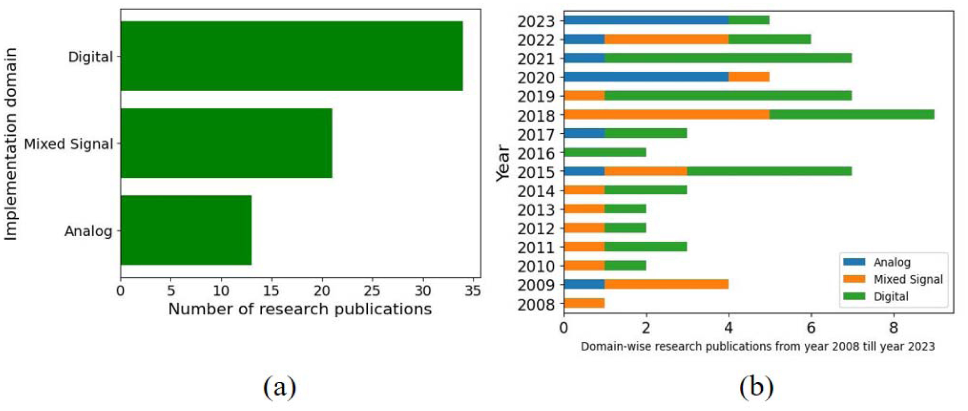
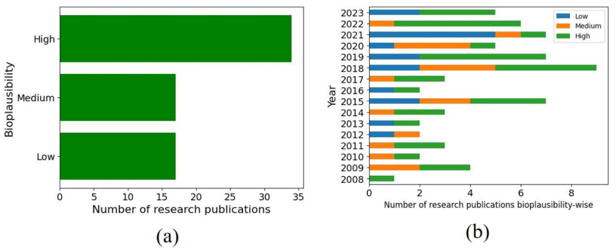
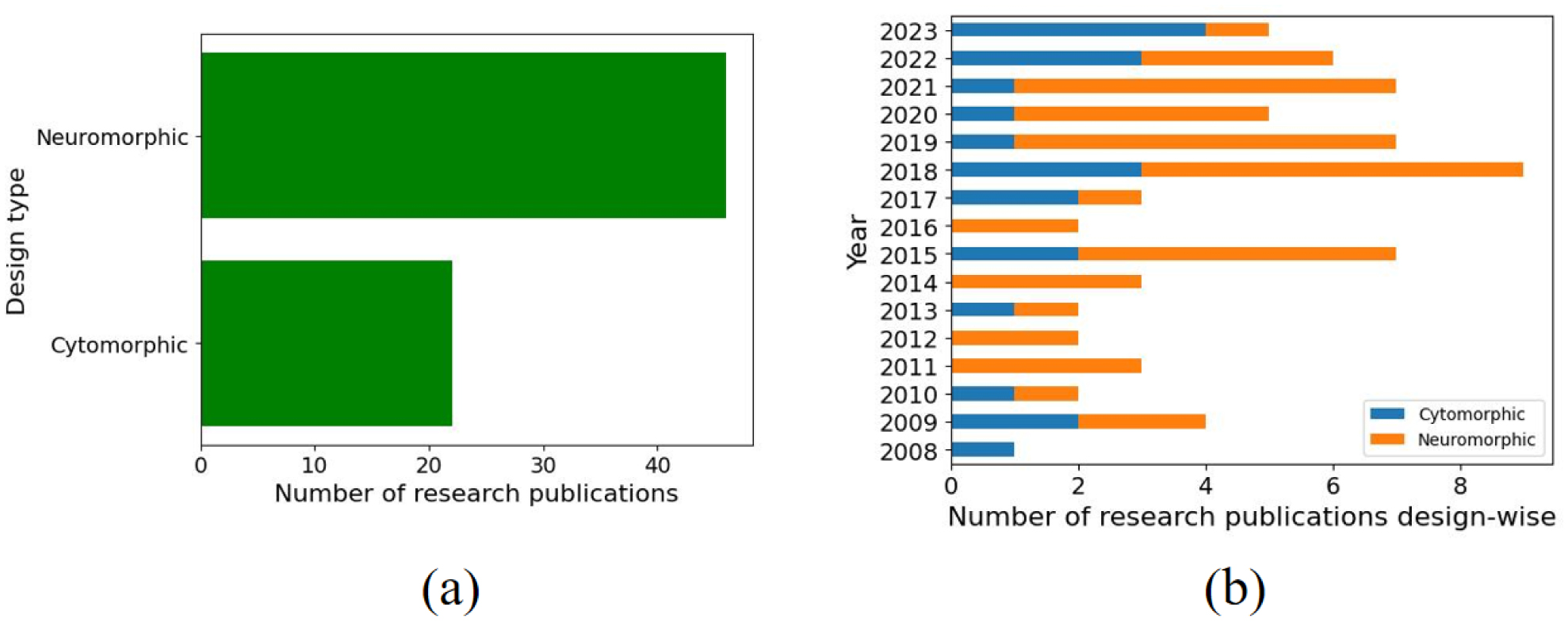
Since the traditional computing paradigm has reached its optimum advancement levels due to saturation in Moore's law and other factors, many researchers are leaning towards other paradigms such as neuromorphic and cytomorphic computing. Thus, in recent decades, the electronic mapping of neural circuits and other biological circuits has attracted widespread attention from various researchers in the field. In the literature on neuromorphic and cytomorphic circuits, we find very rare integrative reviews of the two fields that would suggest a correlation between the two separate but related fields. This survey explores such neuromorphic and cytomorphic designs with biorealistic implementations in the analog, mixed-signal, and digital domains. The trends of the increase in work by eminent researchers in the field suggest an ever-increasing incorporation of biorealism in such designs. We first explored the analog designs in the two fields and find that the earlier designs were mostly based on biophysical mapping of sub-threshold analog circuits with biological time constants, but, later on, some researchers worked with above-threshold complementary metal-oxide semiconductor (CMOS) transistors which allowed time-accelerated implementations with somewhat fewer biophysical aspects incorporated. Analog design facilitates resource-efficient circuits, and we see analog designs still acquired by many eminent researchers in contemporary times. We also see a growing number of researchers taking up analog design with digital programmability and communication techniques as a mixed-signal approach. Then some researchers have resorted to pure digital implementations on account of their flexibility, accuracy and clock speeds, but at the expense of complexity in biorealistic pathways. Digital modeling has gained some traction due to multiplier-less modeling, piecewise linear approximations, and enhanced synaptic communication techniques. In particular, field-programmable gate array-based modeling renders the advantages of low cost, rapid prototyping and accuracy at high speed. Systems based on newer research in neuroscience like the role of astrocytes in neural networks have also been explored. In the past 16 years from 2008 to 2023, where this major shift towards bioplausible design has soared high, we see 50% of the selected publications have used digital design, 31% have used a mixed-signal design, and 19% have used analog design across different levels of bioplausibility. Moreover, we see a growing trend of cytomorphic publications and biorealistic neuromorphic publications over recent years. We have covered many applications of such designs in various emerging fields like synthetic biology, drug testing, neuroprosthetics, and other relevant fields.
Citation: Syeda Ramish Fatima, Maria Waqas. Trends of modeling bio-cellular processes and neural pathways on analog, mixed-signal and digital hardware – a review[J]. AIMS Bioengineering, 2025, 12(2): 177-208. doi: 10.3934/bioeng.2025008
Since the traditional computing paradigm has reached its optimum advancement levels due to saturation in Moore's law and other factors, many researchers are leaning towards other paradigms such as neuromorphic and cytomorphic computing. Thus, in recent decades, the electronic mapping of neural circuits and other biological circuits has attracted widespread attention from various researchers in the field. In the literature on neuromorphic and cytomorphic circuits, we find very rare integrative reviews of the two fields that would suggest a correlation between the two separate but related fields. This survey explores such neuromorphic and cytomorphic designs with biorealistic implementations in the analog, mixed-signal, and digital domains. The trends of the increase in work by eminent researchers in the field suggest an ever-increasing incorporation of biorealism in such designs. We first explored the analog designs in the two fields and find that the earlier designs were mostly based on biophysical mapping of sub-threshold analog circuits with biological time constants, but, later on, some researchers worked with above-threshold complementary metal-oxide semiconductor (CMOS) transistors which allowed time-accelerated implementations with somewhat fewer biophysical aspects incorporated. Analog design facilitates resource-efficient circuits, and we see analog designs still acquired by many eminent researchers in contemporary times. We also see a growing number of researchers taking up analog design with digital programmability and communication techniques as a mixed-signal approach. Then some researchers have resorted to pure digital implementations on account of their flexibility, accuracy and clock speeds, but at the expense of complexity in biorealistic pathways. Digital modeling has gained some traction due to multiplier-less modeling, piecewise linear approximations, and enhanced synaptic communication techniques. In particular, field-programmable gate array-based modeling renders the advantages of low cost, rapid prototyping and accuracy at high speed. Systems based on newer research in neuroscience like the role of astrocytes in neural networks have also been explored. In the past 16 years from 2008 to 2023, where this major shift towards bioplausible design has soared high, we see 50% of the selected publications have used digital design, 31% have used a mixed-signal design, and 19% have used analog design across different levels of bioplausibility. Moreover, we see a growing trend of cytomorphic publications and biorealistic neuromorphic publications over recent years. We have covered many applications of such designs in various emerging fields like synthetic biology, drug testing, neuroprosthetics, and other relevant fields.

| [1] |
Shrestha A, Fang H, Mei Z, et al. (2022) A survey on neuromorphic computing: models and hardware. IEEE Circ Syst Mag 22: 6-35. https://doi.org/10.1109/MCAS.2022.3166331 
|
| [2] |
Mead C, Ismail M (1989) Analog VLSI Implementation of Neural Systems. New York: Springer Science & Business Media. https://doi.org/10.1007/978-1-4613-1639-8
|
| [3] | Frenkel CP, Bol D, Indiveri G Bottom-up and top-down neural processing systems design: Neuromorphic intelligence as the convergence of natural and artificial intelligence (2021) ArXiv Prepr. ArXiv210601288. |
| [4] | Waqas M (2019) Integrated circuit models of bio-cellular networks [PhD thesis]. Karachi: NED University of Engineering and Technology. |
| [5] |
Waqas M, Khurram M, Hasan SMR (2017) Bio-cellular processes modeling on silicon substrate: receptor–ligand binding and Michaelis Menten reaction. Analog Integr Circuits Signal Process 93: 329-340. https://doi.org/10.1007/s10470-017-1044-x
|
| [6] |
Woo SS, Kim J, Sarpeshkar R (2015) A cytomorphic chip for quantitative modeling of fundamental bio-molecular circuits. IEEE Trans Biomed Circuits Syst 9: 527-542. https://doi.org/10.1109/TBCAS.2015.2446431
|
| [7] |
Mead CA, Mahowald MA (1988) A silicon model of early visual processing. Neural networks 1: 91-97. https://doi.org/10.1016/0893-6080(88)90024-X
|
| [8] |
Douglas R, Mahowald M, Mead C (1995) Neuromorphic analogue VLSI. Annu Rev Neurosci 18: 255-281. https://doi.org/10.1146/annurev.ne.18.030195.001351
|
| [9] |
Schemmel J, Bruderle D, Meier K, et al. (2007) Modeling synaptic plasticity within networks of highly accelerated I&F neurons. 2007 IEEE International Symposium on Circuits and Systems (ISCAS) . USA: IEEE 3367-3370. https://doi.org/10.1109/ISCAS.2007.378289
|
| [10] | Schemmel J, Billaudelle S, Dauer P, et al. (2021) Accelerated analog neuromorphic computing. Analog Circuits for Machine Learning, Current/Voltage/Temperature Sensors, and High-speed Communication . Cham: Springer International Publishing 83-102. https://doi.org/10.1007/978-3-030-91741-8_6 |
| [11] |
Maher MAC, Deweerth SP, Mahowald MA, et al. (2002) Implementing neural architectures using analog VLSI circuits. IEEE Circ Syst Mag 36: 643-652. https://doi.org/10.1109/31.31311
|
| [12] | Tanner JE (1986) Integrated Optical Motion Detector (VLSI, Mouse, Image-processing, Smart Sensors). California Institute of Technology. |
| [13] |
Mahowald M, Delbrück T (1988) An analog VLSI implementation of the Marr-Poggio stereo correspondence algorithm. Neural Networks 1: 392. https://doi.org/10.1016/0893-6080(88)90418-2
|
| [14] |
Allen T, Mead C, Faggin F, et al. (1988) Orientation-selective VLSI retina. Visual Communications and Image Processing'88: Third in a Series . SPIE 1040-1046. https://doi.org/10.1117/12.969056
|
| [15] |
Hutchinson J, Koch C, Luo J, et al. (1988) Computing motion using analog and binary resistive networks. Computer 21: 52-63. https://doi.org/10.1109/2.31
|
| [16] |
Lyon RF, Mead C (1988) An analog electronic cochlea. IEEE Trans Acoust Speech Signal Process 36: 1119-1134. https://doi.org/10.1109/29.1639
|
| [17] |
Lazzaro J, Mead CA (1989) A silicon model of auditory localization. Neural Comput 1: 47-57. https://doi.org/10.1162/neco.1989.1.1.47
|
| [18] |
Sarpeshkar R, Lyon RF, Mead CA (1996) An analog VLSI cochlea with new transconductance amplifiers and nonlinear gain control. 1996 IEEE International Symposium on Circuits and Systems. Circuits and Systems Connecting the World. ISCAS 96 . IEEE 292-296. https://doi.org/10.1109/ISCAS.1996.541591
|
| [19] |
Andreou AG, Boahen KA, Pouliquen PO, et al. (1991) Current-mode subthreshold MOS circuits for analog VLSI neural systems. IEEE Trans Neural Networks 2: 205-213. https://doi.org/10.1109/72.80331
|
| [20] |
Moore A, Allman J, Goodman RM (1991) A real-time neural system for color constancy. IEEE Trans Neural Networks 2: 237-247. https://doi.org/10.1109/72.80334
|
| [21] |
Andreou AG, Boahen KA (1994) A 48,000 pixel, 590,000 transistor silicon retina in current-mode subthreshold CMOS. Proceedings of 1994 37th Midwest Symposium on Circuits and Systems . IEEE 97-102. https://doi.org/10.1109/MWSCAS.1994.519199
|
| [22] | Boahen KA, Andreou A A contrast sensitive silicon retina with reciprocal synapses (1991). Available from: https://proceedings.neurips.cc/paper/1991/hash/e836d813fd184325132fca8edcdfb40e-Abstract.html |
| [23] |
Asai T, Ohtani M, Yonezu H (1999) Analog integrated circuits for the Lotka-Volterra competitive neural networks. IEEE Trans Neural Networks 10: 1222-1231. https://doi.org/10.1109/72.788661
|
| [24] |
Mandal S, Zhak SM, Sarpeshkar R (2009) A bio-inspired active radio-frequency silicon cochlea. IEEE J Solid-State Circuits 44: 1814-1828. https://doi.org/10.1109/JSSC.2009.2020465
|
| [25] |
Houssein A, Papadimitriou KI, Drakakis EM (2015) A 1.26 µW cytomimetic IC emulating complex nonlinear mammalian cell cycle dynamics: synthesis, simulation and proof-of-concept measured results. IEEE Trans Biomed Circuits Syst 9: 543-554. https://doi.org/10.1109/TBCAS.2015.2450021
|
| [26] |
Yang Z, Huang Y, Zhu J, et al. (2020) Analog circuit implementation of LIF and STDP models for spiking neural networks. Proceedings of the 2020 on Great Lakes Symposium on VLSI 2020: 469-474. https://doi.org/10.1145/3386263.3406940
|
| [27] | Sharma S, Dhanoa JK (2020) Analog circuit implementation of a cortical neuron. 2020 5th IEEE International Conference on Recent Advances and Innovations in Engineering (ICRAIE) . IEEE 1-5. https://doi.org/10.1109/ICRAIE51050.2020.9358377 |
| [28] |
Ronchini M, Zamani M, Farkhani H, et al. (2020) Tunable voltage-mode subthreshold CMOS neuron. 2020 IEEE Computer Society Annual Symposium on VLSI (ISVLSI) . IEEE 252-257. https://doi.org/10.1109/ISVLSI49217.2020.00053
|
| [29] | Asghar MS, Arslan S, Kim HW (2021) Current multiplier based synapse and neuron circuits for compact SNN chip. 2021 IEEE International Symposium on Circuits and Systems (ISCAS) . IEEE 1-4. https://doi.org/10.1109/ISCAS51556.2021.9401173 |
| [30] |
Oren I, Sinni RA, Daniel R (2023) Ultra-low power electronic circuits inspired by biological genetic processes. Proceedings of the 16th International Joint Conference on Biomedical Engineering Systems and Technologies . Portugal 150-156. https://doi.org/10.5220/0011707800003414
|
| [31] |
Beahm DR, Deng Y, DeAngelo TM, et al. (2023) Drug cocktail formulation via circuit design. IEEE Trans Mol Biol Multi-Scale Commun 9: 28-48. https://doi.org/10.1109/TMBMC.2023.3246928
|
| [32] | Beahm DR, Carvalho JPT, DeAngelo TM, et al. (2023) Lorenzian-chaos-like dynamics in viral-immune cytomorphic chips. 2023 IEEE Biomedical Circuits and Systems Conference (BioCAS) . IEEE 1-5. https://doi.org/10.1109/BioCAS58349.2023.10388975 |
| [33] |
Waqas M, Ainuddin U, Iftikhar U (2022) An analog electronic circuit model for cAMP-dependent pathway-towards creation of Silicon life. AIMS Bioeng 9: 145-162. https://doi.org/10.3934/bioeng.2022011
|
| [34] |
Waqas M, Khurram M, Hasan SMR (2020) Analog electronic circuits to model cooperativity in hill process. Mehran Univ Res J Eng Technol 39: 678-685. https://doi.org/10.22581/muet1982.2004.01
|
| [35] |
Patra T, Chatterjee S, Barman Mandal S (2023) Cytomorphic electrical circuit modeling of tumor suppressor p53 protein pathway. Trans Indian Natl Acad Eng 8: 363-377. https://doi.org/10.1007/s41403-023-00403-0
|
| [36] |
Hasan SMR (2008) A circuit model for bio-chemical cell signaling receptor protein and phosphorylation cascade pathway. 2008 International Conference on Microelectronics . IEEE 284-287. https://doi.org/10.1109/ICM.2008.5393542
|
| [37] |
Hasan SMR (2008) A micro-sequenced CMOS model for cell signaling pathway using G-protein and phosphorylation cascade. 2008 15th International Conference on Mechatronics and Machine Vision in Practice . IEEE 57-62. https://doi.org/10.1109/MMVIP.2008.4749507
|
| [38] |
Hasan SMR (2008) A novel mixed-signal integrated circuit model for DNA-protein regulatory genetic circuits and genetic state machines. IEEE Trans Circuits Syst Regul Pap 55: 1185-1196. https://doi.org/10.1109/TCSI.2008.925632
|
| [39] |
Schemmel J, Brüderle D, Grübl A, et al. (2010) A wafer-scale neuromorphic hardware system for large-scale neural modeling. 2010 ieee international symposium on circuits and systems (iscas) . IEEE 1947-1950. https://doi.org/10.1109/ISCAS.2010.5536970
|
| [40] |
Folowosele F, Harrison A, Cassidy A, et al. (2009) A switched capacitor implementation of the generalized linear integrate-and-fire neuron. 2009 IEEE International Symposium on Circuits and Systems (ISCAS) . IEEE 2149-2152. https://doi.org/10.1109/ISCAS.2009.5118221
|
| [41] |
Folowosele F, Etienne-Cummings R, Hamilton TJ (2009) A CMOS switched capacitor implementation of the Mihalas-Niebur neuron. 2009 IEEE Biomedical Circuits and Systems Conference . IEEE 105-108. https://doi.org/10.1109/BIOCAS.2009.5372072
|
| [42] |
Folowosele F, Hamilton TJ, Etienne-Cummings R (2011) Silicon modeling of the Mihalaş-Niebur neuron. IEEE Trans Neural Network 22: 1915-1927. https://doi.org/10.1109/TNN.2011.2167020
|
| [43] |
Mandal S, Sarpeshkar R (2009) Circuit models of stochastic genetic networks. 2009 IEEE Biomedical Circuits and Systems Conference . IEEE 109-112. https://doi.org/10.1109/BIOCAS.2009.5372073
|
| [44] |
Bamford SA, Murray AF, Willshaw DJ (2012) Spike-timing-dependent plasticity with weight dependence evoked from physical constraints. IEEE Trans Biomed Circuits Syst 6: 385-398. https://doi.org/10.1109/TBCAS.2012.2184285
|
| [45] |
Alam S, Hasan SMR (2013) Integrated circuit modeling of biocellular post-transcription gene mechanisms regulated by microRNA and proteasome. IEEE Trans Circuits Syst Regul Pap 60: 2298-2310. https://doi.org/10.1109/TCSI.2013.2245451
|
| [46] |
Benjamin BV, Gao P, McQuinn E, et al. (2014) Neurogrid: a mixed-analog-digital multichip system for large-scale neural simulations. Proc IEEE 102: 699-716. https://doi.org/10.1109/JPROC.2014.2313565
|
| [47] |
Woo SS, Kim J, Sarpeshkar R (2018) A digitally programmable cytomorphic chip for simulation of arbitrary biochemical reaction networks. IEEE Trans Biomed Circuits Syst 12: 360-378. https://doi.org/10.1109/TBCAS.2017.2781253
|
| [48] |
Kim J, Woo SS, Sarpeshkar R (2018) Fast and precise emulation of stochastic biochemical reaction networks with amplified thermal noise in silicon chips. IEEE Trans Biomed Circuits Syst 12: 379-389. https://doi.org/10.1109/TBCAS.2017.2786306
|
| [49] |
Mayr C, Partzsch J, Noack M, et al. (2015) A biological-realtime neuromorphic system in 28 nm CMOS using low-leakage switched capacitor circuits. IEEE Trans Biomed Circuits Syst 10: 243-254. https://doi.org/10.1109/TBCAS.2014.2379294
|
| [50] |
Rolls ET, Dempere-Marco L, Deco G (2013) Holding multiple items in short term memory: a neural mechanism. PloS one 8: e61078. https://doi.org/10.1371/journal.pone.0061078
|
| [51] | Mayr CG, Partzsch J (2010) Rate and pulse based plasticity governed by local synaptic state variables. Front Synaptic Neurosci 2: 33. https://doi.org/10.3389/fnsyn.2010.00033 |
| [52] | Noack M, Mayr C, Partzsch J, et al. (2012) A switched-capacitor implementation of short-term synaptic dynamics. Proceedings of the 19th International Conference Mixed Design of Integrated Circuits and Systems-MIXDES 2012 . IEEE 214-218. |
| [53] | Noack M, Partzsch J, Mayr C, et al. (2010) Biology-derived synaptic dynamics and optimized system architecture for neuromorphic hardware. Proceedings of the 17th International Conference Mixed Design of Integrated Circuits and Systems-MIXDES 2010 . IEEE 219-224. |
| [54] | Ellguth G, Mayr C, Henker S, et al. (2006) Design techniques for deep submicron CMOS/case study delta-sigma-modulator. Dresdner Arbeitstagung Schaltungs-und Systementwurf 1: 35-40. |
| [55] |
Ishida K, Kanda K, Tamtrakarn A, et al. (2006) Managing subthreshold leakage in charge-based analog circuits with low-V/sub TH/transistors by analog T-switch (AT-switch) and super cut-off CMOS (SCCMOS). IEEE J Solid-State Circuits 41: 859-867. https://doi.org/10.1109/JSSC.2006.870761
|
| [56] |
Aamir SA, Müller P, Kiene G, et al. (2018) A mixed-signal structured AdEx neuron for accelerated neuromorphic cores. IEEE Trans Biomed Circuits Syst 12: 1027-1037. https://doi.org/10.1109/TBCAS.2018.2848203
|
| [57] |
Brette R, Gerstner W (2005) Adaptive exponential integrate-and-fire model as an effective description of neuronal activity. J Neurophysiol 94: 3637-3642. https://doi.org/10.1152/jn.00686.2005
|
| [58] |
Touboul J, Brette R (2008) Dynamics and bifurcations of the adaptive exponential integrate-and-fire model. Biol Cybern 99: 319-334. https://doi.org/10.1007/s00422-008-0267-4
|
| [59] | Jolivet R, Rauch A, Lüscher H R, et al. Integrate-and-fire models with adaptation are good enough (2005). Available from: https://proceedings.neurips.cc/paper/2005/hash/42a6845a557bef704ad8ac9cb4461d43-Abstract.html |
| [60] |
Aamir SA, Stradmann Y, Müller P, et al. (2018) An accelerated LIF neuronal network array for a large-scale mixed-signal neuromorphic architecture. IEEE Trans Circuits Syst Regul Pap 65: 4299-4312. https://doi.org/10.1109/TCSI.2018.2840718
|
| [61] |
Neckar A, Fok S, Benjamin BV, et al. (2018) Braindrop: a mixed-signal neuromorphic architecture with a dynamical systems-based programming model. Proc IEEE 107: 144-164. https://doi.org/10.1109/JPROC.2018.2881432
|
| [62] |
Teo JJY, Weiss R, Sarpeshkar R (2019) An artificial tissue homeostasis circuit designed via analog circuit techniques. IEEE Trans Biomed Circuits Syst 13: 540-553. https://doi.org/10.1109/TBCAS.2019.2907074
|
| [63] |
Beahm DR, Deng Y, Riley TG, et al. (2021) Cytomorphic electronic systems: a review and perspective. IEEE Nanotechnol Mag 15: 41-53. https://doi.org/10.1109/MNANO.2021.3113192
|
| [64] |
Rubino A, Livanelioglu C, Qiao N, et al. (2020) Ultra-low-power FDSOI neural circuits for extreme-edge neuromorphic intelligence. IEEE Trans Circuits Syst Regul Pap 68: 45-56. https://doi.org/10.1109/TCSI.2020.3035575
|
| [65] |
Jo Y, Mun K, Jeong Y, et al. (2022) A poisson process generator based on multiple thermal noise amplifiers for parallel stochastic simulation of biochemical reactions. Electronics 11: 1039. https://doi.org/10.3390/electronics11071039
|
| [66] |
Zhao H, Sarpeshkar R, Mandal S (2022) A compact and power-efficient noise generator for stochastic simulations. IEEE Trans Circuits Syst Regul Pap 70: 3-16. https://doi.org/10.1109/TCSI.2022.3199561
|
| [67] |
Wang M, Yan B, Hu J, et al. (2011) Simulation of large neuronal networks with biophysically accurate models on graphics processors. The 2011 International Joint Conference on Neural Networks . IEEE 3184-3193. https://doi.org/10.1109/IJCNN.2011.6033643
|
| [68] |
Igarashi J, Shouno O, Fukai T, et al. (2011) Real-time simulation of a spiking neural network model of the basal ganglia circuitry using general purpose computing on graphics processing units. Neural Netw 24: 950-960. https://doi.org/10.1016/j.neunet.2011.06.008
|
| [69] |
Yamaguchi Y, Azuma R, Konagaya A, et al. (2003) An approach for the high speed Monte Carlo simulation with FPGA-toward a whole cell simulation. 2003 46th Midwest Symposium on Circuits and Systems . IEEE 364-367. https://doi.org/10.1109/MWSCAS.2003.1562294
|
| [70] |
Yamaguchi Y, Maruyama T, Azuma R, et al. (2007) Mesoscopic-level simulation of dynamics and interactions of biological molecules using monte carlo simulation. J VLSI Signal Process Syst Signal Image Video Technol 48: 287-299. https://doi.org/10.1007/s11265-007-0072-7
|
| [71] |
Mak TST, Rachmuth G, Lam KP, et al. (2006) A component-based FPGA design framework for neuronal ion channel dynamics simulations. IEEE Trans Neural Syst Rehabil Eng 14: 410-418. https://doi.org/10.1109/TNSRE.2006.886727
|
| [72] |
Graas EL, Brown EA, Lee RH (2004) An FPGA-based approach to high-speed simulation of conductance-based neuron models. Neuroinformatics 2: 417-435. https://doi.org/10.1385/NI:2:4:417
|
| [73] | Mak TS, Rachmuth G, Lam KP, et al. (2005) Field programmable gate array implementation of neuronal ion channel dynamics. Conference Proceedings. 2nd International IEEE EMBS Conference on Neural Engineering . IEEE 144-148. https://doi.org/10.1109/CNE.2005.1419574 |
| [74] | Weinstein RK, Lee RH (2005) Design of high performance physiologically-complex motoneuron models in fpgas. Conference Proceedings. 2nd International IEEE EMBS Conference on Neural Engineering . IEEE 526-528. https://doi.org/10.1109/CNE.2005.1419675 |
| [75] |
Weinstein RK, Lee RH (2005) Architectures for high-performance FPGA implementations of neural models. J Neural Eng 3: 21. https://doi.org/10.1088/1741-2560/3/1/003
|
| [76] |
Hasan SMR (2010) A digital cmos sequential circuit model for bio-cellular adaptive immune response pathway using phagolysosomic digestion: a digital phagocytosis engine. J Biomed Sci Eng 3: 470-475. https://doi.org/10.4236/jbise.2010.35065
|
| [77] |
Weinstein RK, Reid MS, Lee RH (2007) Methodology and design flow for assisted neural-model implementations in FPGAs. IEEE Trans Neural Syst Rehabil Eng 15: 83-93. https://doi.org/10.1109/TNSRE.2007.891379
|
| [78] |
Soleimani H, Ahmadi A, Bavandpour M (2012) Biologically inspired spiking neurons: piecewise linear models and digital implementation. IEEE Trans Circuits Syst Regul Pap 59: 2991-3004. https://doi.org/10.1109/TCSI.2012.2206463
|
| [79] |
Cassidy AS, Georgiou J, Andreou AG (2013) Design of silicon brains in the nano-CMOS era: spiking neurons, learning synapses and neural architecture optimization. Neural Netw 45: 4-26. https://doi.org/10.1016/j.neunet.2013.05.011
|
| [80] |
Nazari S, Faez K, Karami E, et al. (2014) A digital neurmorphic circuit for a simplified model of astrocyte dynamics. Neurosci Lett 582: 21-26. https://doi.org/10.1016/j.neulet.2014.07.055
|
| [81] |
Smaragdos G, Isaza S, van Eijk MF, et al. (2014) FPGA-based biophysically-meaningful modeling of olivocerebellar neurons. Proceedings of the 2014 ACM/SIGDA international symposium on Field-programmable gate arrays 2014: 89-98. https://doi.org/10.1145/2554688.2554790
|
| [82] |
Moctezuma JC, McGeehan JP, Nunez-Yanez JL (2015) Biologically compatible neural networks with reconfigurable hardware. Microprocess Microsyst 39: 693-703. https://doi.org/10.1016/j.micpro.2015.09.003
|
| [83] |
Pinsky PF, Rinzel J (1994) Intrinsic and network rhythmogenesis in a reduced Traub model for CA3 neurons. J Comput Neurosci 1: 39-60. https://doi.org/10.1007/BF00962717
|
| [84] |
Yang S, Wang J, Zhao A, et al. (2016) A multi-FPGA embedded system for the emulation of modular small-world network with real time dynamics. 2016 12th World Congress on Intelligent Control and Automation (WCICA) . IEEE 2198-2203. https://doi.org/10.1109/WCICA.2016.7578502
|
| [85] |
Deng B, Zhu Z, Yang S, et al. (2016) FPGA implementation of motifs-based neuronal network and synchronization analysis. Phys Stat Mech Its Appl 451: 388-402. https://doi.org/10.1016/j.physa.2016.01.052
|
| [86] |
Rahimian E, Zabihi S, Amiri M, et al. (2017) Digital implementation of the two-compartmental Pinsky-Rinzel pyramidal neuron model. IEEE Trans Biomed Circuits Syst 12: 47-57. https://doi.org/10.1109/TBCAS.2017.2753541
|
| [87] |
Yang S, Wang J, Li S, et al. (2015) Cost-efficient FPGA implementation of basal ganglia and their Parkinsonian analysis. Neural Netw 71: 62-75. https://doi.org/10.1016/j.neunet.2015.07.017
|
| [88] |
Luo J, Coapes G, Mak T, et al. (2015) Real-time simulation of passage-of-time encoding in cerebellum using a scalable FPGA-based system. IEEE Trans Biomed Circuits Syst 10: 742-753. https://doi.org/10.1109/TBCAS.2015.2460232
|
| [89] |
Akopyan F, Sawada J, Cassidy A, et al. (2015) Truenorth: Design and tool flow of a 65 mw 1 million neuron programmable neurosynaptic chip. IEEE Trans Comput-Aided Des Integr Circuits Syst 34: 1537-1557. https://doi.org/10.1109/TCAD.2015.2474396
|
| [90] |
Soleimani H, Drakakis EM (2017) A compact synchronous cellular model of nonlinear calcium dynamics: Simulation and FPGA synthesis results. IEEE Trans Biomed Circuits Syst 11: 703-713. https://doi.org/10.1109/TBCAS.2016.2636183
|
| [91] |
Davies M, Srinivasa N, Lin TH, et al. (2018) Loihi: a neuromorphic manycore processor with on-chip learning. Ieee Micro 38: 82-99. https://doi.org/10.1109/MM.2018.112130359
|
| [92] |
Orchard G, Frady EP, Rubin DBD, et al. (2021) Efficient neuromorphic signal processing with loihi 2. 2021 IEEE Workshop on Signal Processing Systems (SiPS) . IEEE 254-259. https://doi.org/10.1109/SiPS52927.2021.00053
|
| [93] |
Soleimani H, Drakakis EM (2018) A low-power digital IC emulating intracellular calcium dynamics. Int J Circuit Theory Appl 46: 1929-1939. https://doi.org/10.1002/cta.2514
|
| [94] |
Faramarzi F, Azad F, Amiri M, et al. (2019) A neuromorphic digital circuit for neuronal information encoding using astrocytic calcium oscillations. Front Neurosci 13: 998. https://doi.org/10.3389/fnins.2019.00998
|
| [95] |
Yang S, Wang J, Deng B, et al. (2018) Real-time neuromorphic system for large-scale conductance-based spiking neural networks. IEEE Trans Cybern 49: 2490-2503. https://doi.org/10.1109/TCYB.2018.2823730
|
| [96] |
Yang S, Wang J, Lin Q, et al. (2018) Cost-efficient FPGA implementation of a biologically plausible dopamine neural network and its application. Neurocomputing 314: 394-408. https://doi.org/10.1016/j.neucom.2018.07.006
|
| [97] |
Hao X, Yang S, Wang J, et al. (2019) Efficient implementation of cerebellar purkinje cell with the CORDIC algorithm on LaCSNN. Front Neurosci 13: 1078. https://doi.org/10.3389/fnins.2019.01078
|
| [98] |
Hao J, Hao X, Wang J, et al. (2019) Behavior of a hippocampal spiking network and FPGA implementation. 2019 Chinese Control Conference (CCC) . IEEE 8433-8438. https://doi.org/10.23919/ChiCC.2019.8866461
|
| [99] |
Yang S, Wang J, Deng B, et al. (2019) Digital implementation of the retinal spiking neural network under light stimulation. 2019 9th International IEEE/EMBS Conference on Neural Engineering (NER) . IEEE 542-545. https://doi.org/10.1109/NER.2019.8716932
|
| [100] |
George R, Chiappalone M, Giugliano M, et al. (2020) Plasticity and adaptation in neuromorphic biohybrid systems. Iscience 23: 101589. https://doi.org/10.1016/j.isci.2020.101589
|
| [101] |
Yang S, Deng B, Wang J, et al. (2019) Scalable digital neuromorphic architecture for large-scale biophysically meaningful neural network with multi-compartment neurons. IEEE Trans Neural Netw Learn Syst 31: 148-162. https://doi.org/10.1109/TNNLS.2019.2899936
|
| [102] |
Kuang Z, Wang J, Yang S, et al. (2019) Digital implementation of the spiking neural network and its digit recognition. 2019 Chinese Control And Decision Conference (CCDC) . IEEE 3621-3625. https://doi.org/10.1109/CCDC.2019.8832952
|
| [103] | Seyedbarhagh M, Ahmadi A, Ahmadi M (2021) Digital Realization for Ca2+ Waves Stimulated by the (mGlu5) Receptors. 2021 International Symposium on Signals, Circuits and Systems (ISSCS) . IEEE 1-4. https://doi.org/10.1109/ISSCS52333.2021.9497380 |
| [104] |
Yang S, Wang J, Deng B, et al. (2021) Neuromorphic context-dependent learning framework with fault-tolerant spike routing. IEEE Trans Neural Netw Learn Syst 33: 7126-7140. https://doi.org/10.1109/TNNLS.2021.3084250
|
| [105] |
Deng B, Fan Y, Wang J, et al. (2021) Reconstruction of a fully paralleled auditory spiking neural network and FPGA implementation. IEEE Trans Biomed Circuits Syst 15: 1320-1331. https://doi.org/10.1109/TBCAS.2021.3122549
|
| [106] | Yang S, Kuang Z, Deng B, et al. (2021) Reconstruction of brain-inspired visual spiking neural network on bicoss. 2021 IEEE 3rd International Conference on Frontiers Technology of Information and Computer (ICFTIC) . IEEE 612-616. https://doi.org/10.1109/ICFTIC54370.2021.9647242 |
| [107] |
Yang S, Wang J, Hao X, et al. (2022) BiCoSS: toward large-scale cognition brain with multigranular neuromorphic architecture. IEEE Trans Neural Netw Learn Syst 33: 2801-2815. https://doi.org/10.1109/TNNLS.2020.3045492
|
| [108] |
Yang S, Wang J, Zhang N, et al. (2022) CerebelluMorphic: large-scale neuromorphic model and architecture for supervised motor learning. IEEE Trans Neural Netw Learn Syst 33: 4398-4412. https://doi.org/10.1109/TNNLS.2021.3057070
|
| [109] |
Acharya M, Dey S, Chakrabarti A, et al. (2023) FPGA based library subset design for different biochemical reactions involved in a cell. Sādhanā 48: 264. https://doi.org/10.1007/s12046-023-02314-w
|
| [110] | Soma BM, Moumita A, Samik B, et al. (2021) FPGA implementation of different stochastic biochemical reactions involved in a cell. 2021 25th International Symposium on VLSI Design and Test (VDAT) . IEEE 1-4. https://doi.org/10.1109/VDAT53777.2021.9601094 |
| [111] |
Daniel R, Rubens JR, Sarpeshkar R, et al. (2013) Synthetic analog computation in living cells. Nature 497: 619-623. https://doi.org/10.1038/nature12148
|
| [112] | Sarpeshkar R (2014) Analog synthetic biology. Philos Trans R Soc Math Phys Eng Sci 372: 20130110. https://doi.org/10.1098/rsta.2013.0110 |
| [113] |
Teo JJY, Woo SS, Sarpeshkar R (2015) Synthetic biology: a unifying view and review using analog circuits. IEEE Trans Biomed Circuits Syst 9: 453-474. https://doi.org/10.1109/TBCAS.2015.2461446
|
Figures(3) / Tables(5)

Syeda Ramish Fatima, Maria Waqas. Trends of modeling bio-cellular processes and neural pathways on analog, mixed-signal and digital hardware – a review[J]. AIMS Bioengineering, 2025, 12(2): 177-208. doi: 10.3934/bioeng.2025008


 DownLoad: