Gestational diabetes mellitus (GDM), characterized by glucose intolerance during pregnancy, poses substantial health risks for both mothers and infants due to the interplay of insulin resistance and β-cell dysfunction. Molecular biomarkers, including SNPs, microRNAs (miRNAs), and proteins, have been linked to GDM development during pregnancy. Notably, miRNA-mediated regulation of gene expression holds pivotal roles in metabolic disorders. This study aims to identify diagnostic biomarkers for GDM and establish a diagnostic model.
Firstly, gene expression data from GDM samples (N = 9) and normal samples (N = 9) were sourced from the Gene Expression Omnibus (GEO) database. Subsequently, the limma package was employed to discern differentially expressed genes (DEGs), with subsequent functional and enrichment analyses executed using the clusterProfiler package. A comprehensive exploration of genes significantly correlated with GDM was undertaken via weighted gene co-expression network analysis (WGCNA). The construction of a protein-protein interaction (PPI) network was facilitated by STRING, while visualization of hub genes was achieved through Cytoscape. Moreover, the miRNA-mRNA network was established using StarBase. Concurrently, immune infiltration significantly correlated with hub genes was identified.
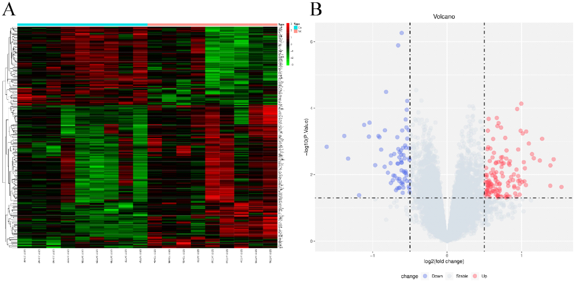
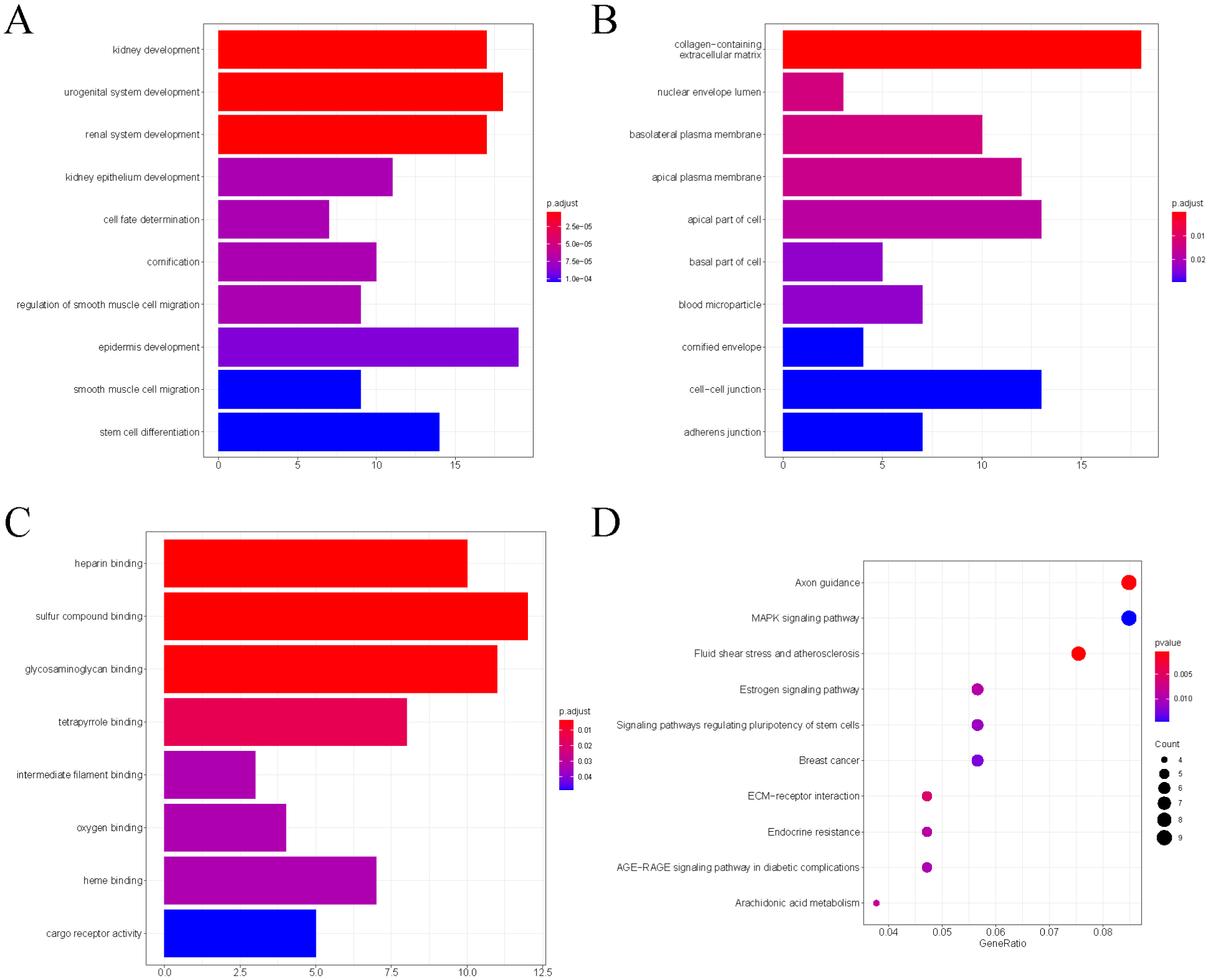
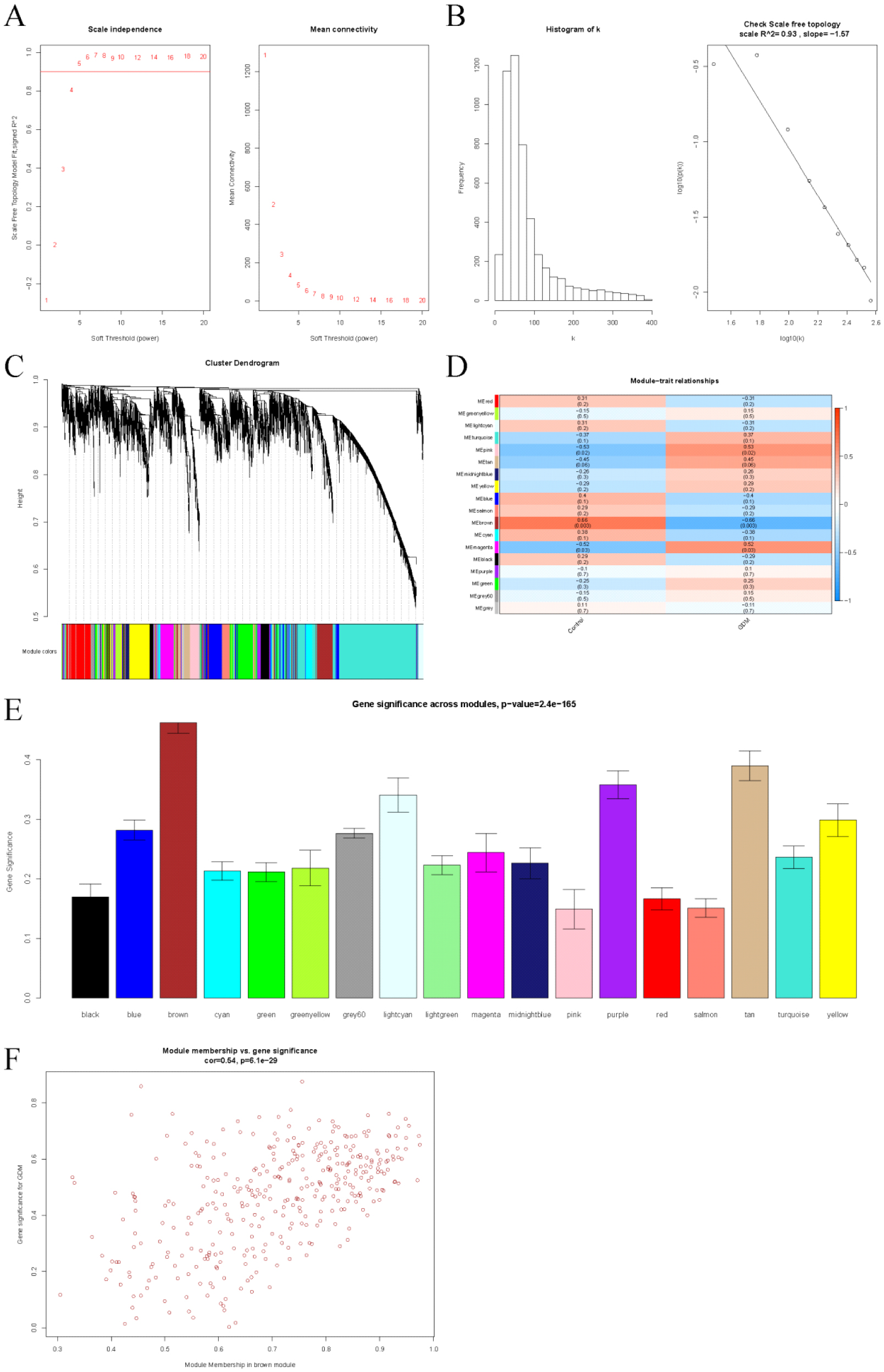
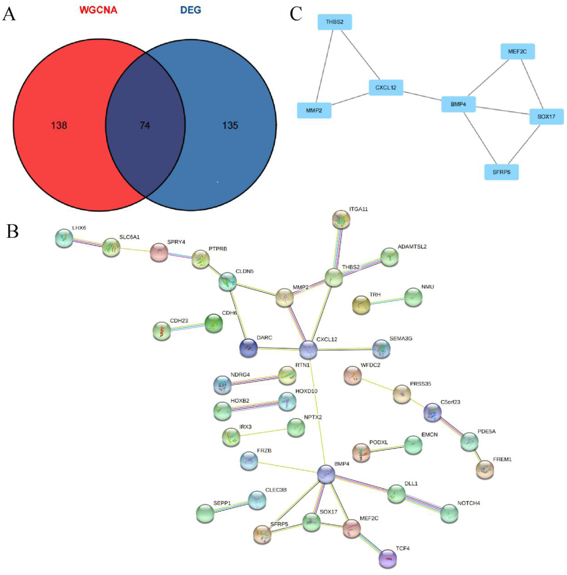
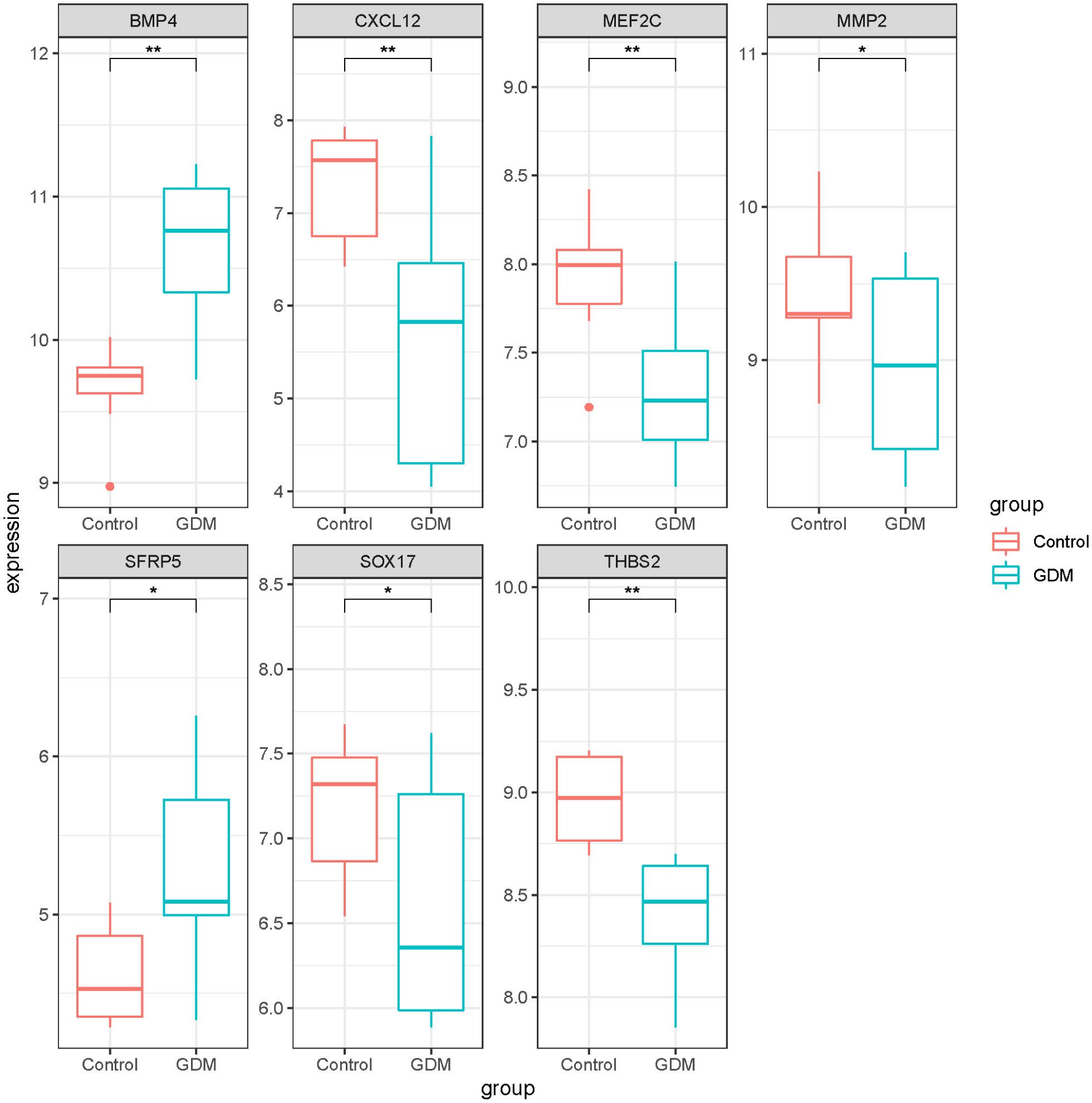
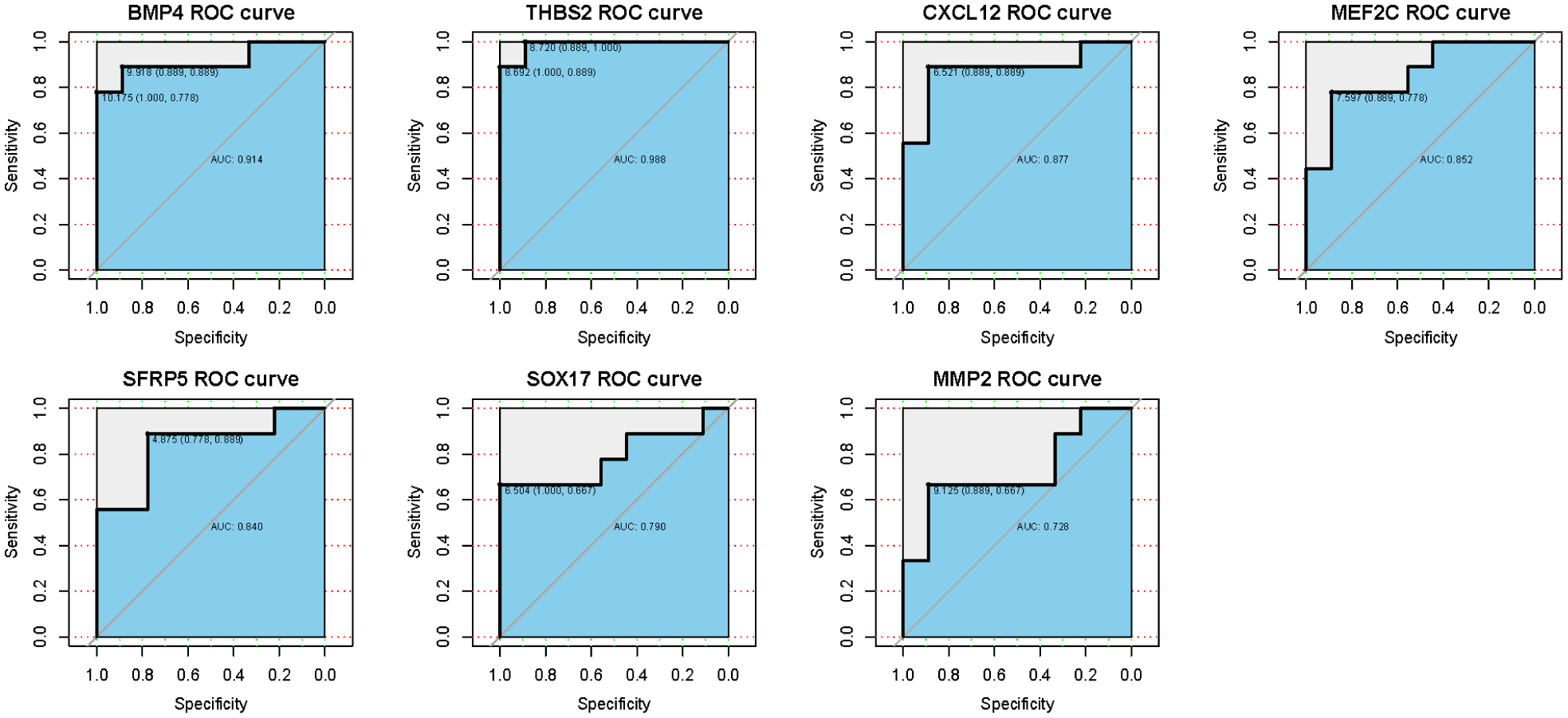
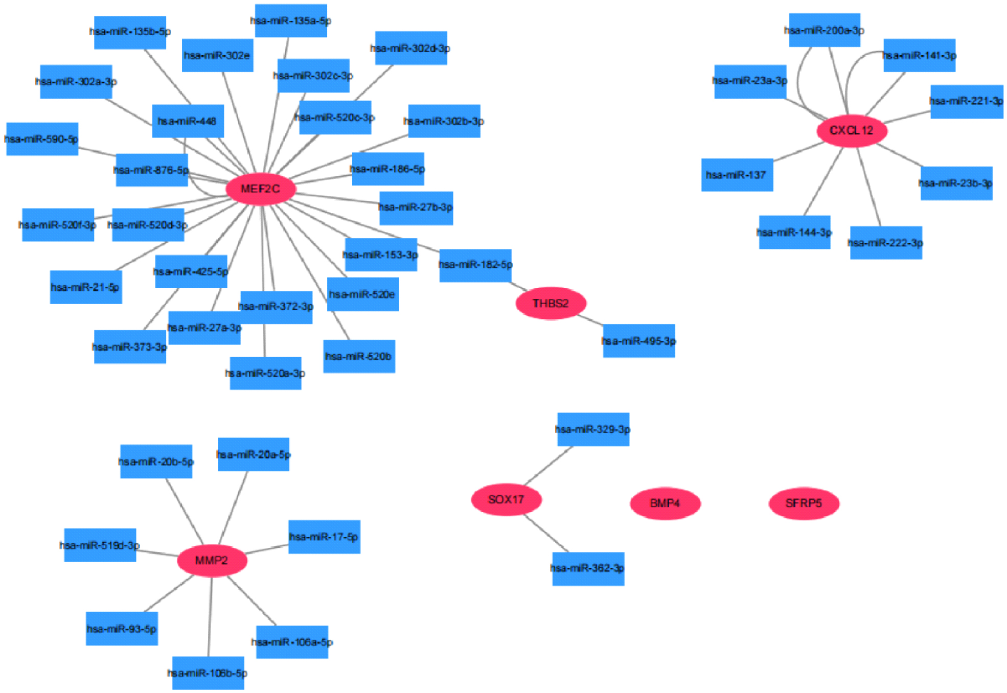
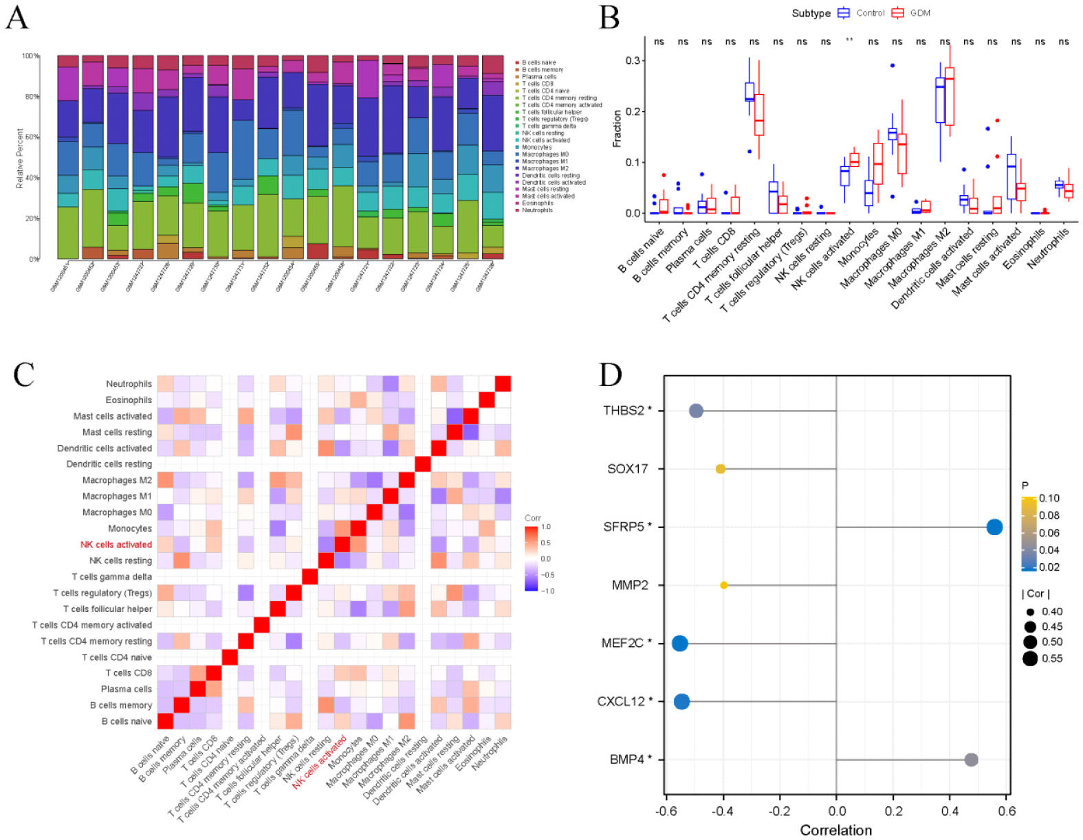
In this study, 209 DEGs between normal and GDM samples were identified, and these genes were associated with collagen containing extracellular matrix heparin binding and axon guidance, etc. Then, 18 modules were identified by WGCNA and the brown module including 212 genes had a significantly negative correlation with GDM (r = −0.66, P = 0.003). Additionally, five low gene expressions (CXCL12, MEF2C, MMP2, SOX17 and THBS2) and two high gene expressions (BMP4 and SFRP5) were identified as GDM related hub genes. Moreover, hub genes regulated by alternations of miRNAs were established and three hub genes (CXCL12, MEF2C and THBS2) were negatively correlated with activated Natural Killer (NK) cells while two hub genes (BMP4 and SFRP5) were positively correlated with activated NK cells.
This study offers novel hub genes that could contribute to the diagnostic approach for GDM, potentially shedding light on the intricate mechanisms underpinning GDM's developmental pathways.
Citation: Xuemei XIA, Xuemei HU. Identification of diagnostic biomarkers of gestational diabetes mellitus based on transcriptome gene expression and alternations of microRNAs[J]. AIMS Bioengineering, 2023, 10(3): 202-217. doi: 10.3934/bioeng.2023014
Gestational diabetes mellitus (GDM), characterized by glucose intolerance during pregnancy, poses substantial health risks for both mothers and infants due to the interplay of insulin resistance and β-cell dysfunction. Molecular biomarkers, including SNPs, microRNAs (miRNAs), and proteins, have been linked to GDM development during pregnancy. Notably, miRNA-mediated regulation of gene expression holds pivotal roles in metabolic disorders. This study aims to identify diagnostic biomarkers for GDM and establish a diagnostic model.
Firstly, gene expression data from GDM samples (N = 9) and normal samples (N = 9) were sourced from the Gene Expression Omnibus (GEO) database. Subsequently, the limma package was employed to discern differentially expressed genes (DEGs), with subsequent functional and enrichment analyses executed using the clusterProfiler package. A comprehensive exploration of genes significantly correlated with GDM was undertaken via weighted gene co-expression network analysis (WGCNA). The construction of a protein-protein interaction (PPI) network was facilitated by STRING, while visualization of hub genes was achieved through Cytoscape. Moreover, the miRNA-mRNA network was established using StarBase. Concurrently, immune infiltration significantly correlated with hub genes was identified.
In this study, 209 DEGs between normal and GDM samples were identified, and these genes were associated with collagen containing extracellular matrix heparin binding and axon guidance, etc. Then, 18 modules were identified by WGCNA and the brown module including 212 genes had a significantly negative correlation with GDM (r = −0.66, P = 0.003). Additionally, five low gene expressions (CXCL12, MEF2C, MMP2, SOX17 and THBS2) and two high gene expressions (BMP4 and SFRP5) were identified as GDM related hub genes. Moreover, hub genes regulated by alternations of miRNAs were established and three hub genes (CXCL12, MEF2C and THBS2) were negatively correlated with activated Natural Killer (NK) cells while two hub genes (BMP4 and SFRP5) were positively correlated with activated NK cells.
This study offers novel hub genes that could contribute to the diagnostic approach for GDM, potentially shedding light on the intricate mechanisms underpinning GDM's developmental pathways.

| [1] |
Plows JF, Stanley JL, Baker PN, et al. (2018) The pathophysiology of gestational diabetes mellitus. Int J Mol Sci 19: 3342. https://doi.org/10.3390/ijms19113342 
|
| [2] |
Szmuilowicz ED, Josefson JL, Metzger BE (2019) Gestational diabetes mellitus. Endocrinol Metab Clin North Am 48: 479-493. https://doi.org/10.1016/j.ecl.2019.05.001
|
| [3] |
Mack LR, Tomich PG (2017) Gestational diabetes: diagnosis, classification, and clinical care. Obstet Gynecol Clin North Am 44: 207-217. https://doi.org/10.1016/j.ogc.2017.02.002
|
| [4] |
Simmons D (2019) GDM and nutrition-answered and unanswered questions-there's more work to do!. Nutrients 11: 1940. https://doi.org/10.3390/nu11081940
|
| [5] |
Kramer CK, Campbell S, Retnakaran R (2019) Gestational diabetes and the risk of cardiovascular disease in women: a systematic review and meta-analysis. Diabetologia 62: 905-914. https://doi.org/10.1007/s00125-019-4840-2
|
| [6] |
Mardente S, Zicari A, Santangelo C, et al. (2020) Non-coding RNA: Role in gestational diabetes pathophysiology and complications. Int J Mol Sci 21: 4020. https://doi.org/10.3390/ijms21114020
|
| [7] |
Kang L, Li HY, Ou HY, et al. (2020) Role of placental fibrinogen-like protein 1 in gestational diabetes. Transl Res 218: 73-80. https://doi.org/10.1016/j.trsl.2020.01.001
|
| [8] |
Yu Z, Liu J, Zhang R, et al. (2017) IL-37 and 38 signalling in gestational diabetes. J Reprod Immunol 124: 8-14. https://doi.org/10.1016/j.jri.2017.09.011
|
| [9] |
Mosavat M, Omar SZ, Jamalpour S, et al. (2020) Serum glucose-dependent insulinotropic polypeptide (GIP) and glucagon-like peptide-1 (GLP-1) in association with the risk of gestational diabetes: a prospective case-control study. J Diabetes Res 2020: 9072492. https://doi.org/10.1155/2020/9072492
|
| [10] |
Dias S, Pheiffer C (2018) Molecular biomarkers for gestational diabetes mellitus. Int J Mol Sci 19: 2926. https://doi.org/10.3390/ijms19102926
|
| [11] |
Gillet V, Ouellet A, Stepanov Y, et al. (2019) miRNA profiles in extracellular vesicles from serum early in pregnancies complicated by gestational diabetes mellitus. J Clin Endocrinol Metab 104: 5157-5169. https://doi.org/10.1210/jc.2018-02693
|
| [12] |
Yoffe L, Polsky A, Gilam A, et al. (2019) Early diagnosis of gestational diabetes mellitus using circulating microRNAs. Eur J Endocrinol 181: 565-577. https://doi.org/10.1530/EJE-19-0206
|
| [13] |
Zhu W, Shen Y, Liu J, et al. (2020) Epigenetic alternations of microRNAs and DNA methylation contribute to gestational diabetes mellitus. J Cell Mol Med 24: 13899-13912. https://doi.org/10.1111/jcmm.15984
|
| [14] |
Chen M, Yan J (2020) Identification of hub-methylated differentially expressed genes in patients with gestational diabetes mellitus by multi-omic WGCNA basing epigenome-wide and transcriptome-wide profiling. J Cell Biochem 121: 3173-3184. https://doi.org/10.1002/jcb.29584
|
| [15] |
Li E, Luo T, Wang Y (2019) Identification of diagnostic biomarkers in patients with gestational diabetes mellitus based on transcriptome gene expression and methylation correlation analysis. Reprod Biol Endocrinol 17: 112. https://doi.org/10.1186/s12958-019-0556-x
|
| [16] |
Wang Y, Wang Z, Zhang H (2018) Identification of diagnostic biomarker in patients with gestational diabetes mellitus based on transcriptome-wide gene expression and pattern recognition. J Cell Biochem 120: 1503-1510. https://doi.org/10.1002/jcb.27279
|
| [17] |
He L, Wang X, Jin Y, et al. (2021) Identification and validation of the miRNA-mRNA regulatory network in fetoplacental arterial endothelial cells of gestational diabetes mellitus. Bioengineered 12: 3503-3515. https://doi.org/10.1080/21655979.2021.1950279
|
| [18] | Liu Y, Geng H, Duan B, et al. (2021) Identification of diagnostic CpG signatures in Patients with gestational diabetes mellitus via epigenome-wide association study integrated with machine learning. Biomed Res Int 2021: 1984690. https://doi.org/10.1155/2021/1984690 |
| [19] | Pan X, Jin X, Wang J, et al. (2021) Placenta inflammation is closely associated with gestational diabetes mellitus. Am J Transl Res 13: 4068-4079. |
| [20] | He Y, Bai J, Liu P, et al. (2017) miR-494 protects pancreatic β-cell function by targeting PTEN in gestational diabetes mellitus. EXCLI J 16: 1297-1307. https://doi.org/10.17179/excli2017-491 |
| [21] | Liu Z, Yu X, Tong C, et al. (2019) Renal dysfunction in a mouse model of GDM is prevented by metformin through MAPKs. Mol Med Rep 19: 4491-4499. https://doi.org/10.3892/mmr.2019.10060 |
| [22] |
Liu H, Liu A, Kaminga AC, et al. (2022) Chemokines in gestational diabetes mellitus. Front Immunol 13: 705852. https://doi.org/10.3389/fimmu.2022.705852
|
| [23] |
Darakhshan S, Fatehi A, Hassanshahi G, et al. (2019) Serum concentration of angiogenic (CXCL1, CXCL12) and angiostasis (CXCL9, CXCL10) CXC chemokines are differentially altered in normal and gestational diabetes mellitus associated pregnancies. J Diabetes Metab Disord 18: 371-378. https://doi.org/10.1007/s40200-019-00421-2
|
| [24] |
Wu G, Li R, Tong C, et al. (2019) Non-invasive prenatal testing reveals copy number variations related to pregnancy complications. Mol Cytogenet 12: 38. https://doi.org/10.1186/s13039-019-0451-3
|
| [25] |
Bartoszewicz Z, Wielgos M, Wielgos M, et al. (2021) Maternal and neonatal serum expression of the vascular growth factors in hyperglycemia in pregnancy. J Matern Fetal Neonatal Med 34: 1673-1678. https://doi.org/10.1080/14767058.2019.1639666
|
| [26] |
Damasceno AA, Carvalho CP, Santos EM, et al. (2014) Effects of maternal diabetes on male offspring: high cell proliferation and increased activity of MMP-2 in the ventral prostate. Cell Tissue Res 358: 257-269. https://doi.org/10.1007/s00441-014-1941-6
|
| [27] |
Cai B, Du J (2021) Role of bone morphogenic protein-4 in gestational diabetes mellitus-related hypertension. Exp Ther Med 22: 762. https://doi.org/10.3892/etm.2021.10194
|
| [28] | De Luccia TPB, Pendeloski KPT (2020) Unveiling the pathophysiology of gestational diabetes: Studies on local and peripheral immune cells. Scand J Immunol 91: e12860. https://doi.org/10.1111/sji.12860 |
| [29] | Hara Cde C, França EL, Fagundes DL, et al. (2016) Characterization of natural killer cells and cytokines in maternal placenta and fetus of diabetic mothers. J Immunol Res 2016: 7154524. https://doi.org/10.1155/2016/7154524 |
Figures(9)

Xuemei XIA, Xuemei HU. Identification of diagnostic biomarkers of gestational diabetes mellitus based on transcriptome gene expression and alternations of microRNAs[J]. AIMS Bioengineering, 2023, 10(3): 202-217. doi: 10.3934/bioeng.2023014


 DownLoad: