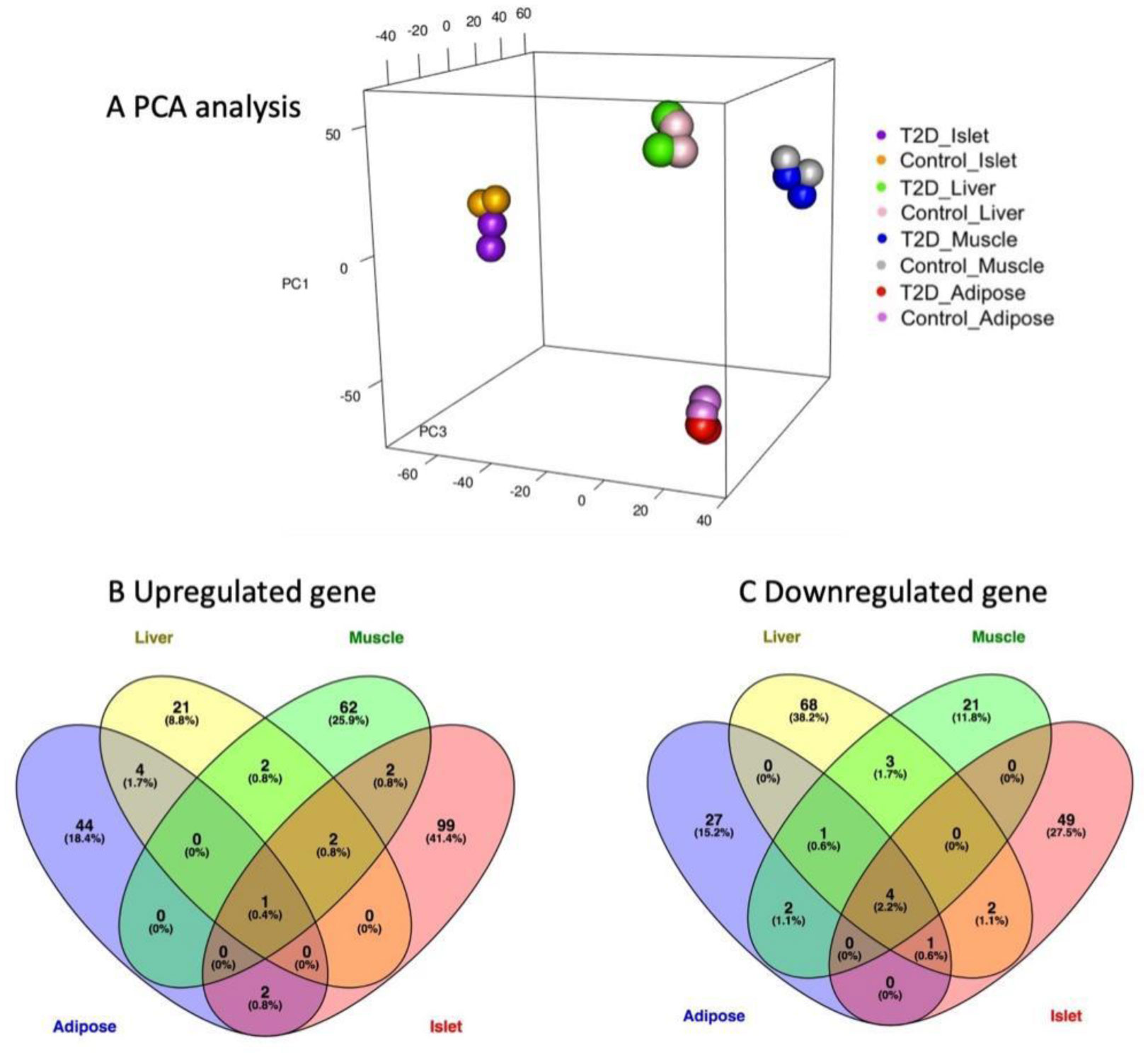
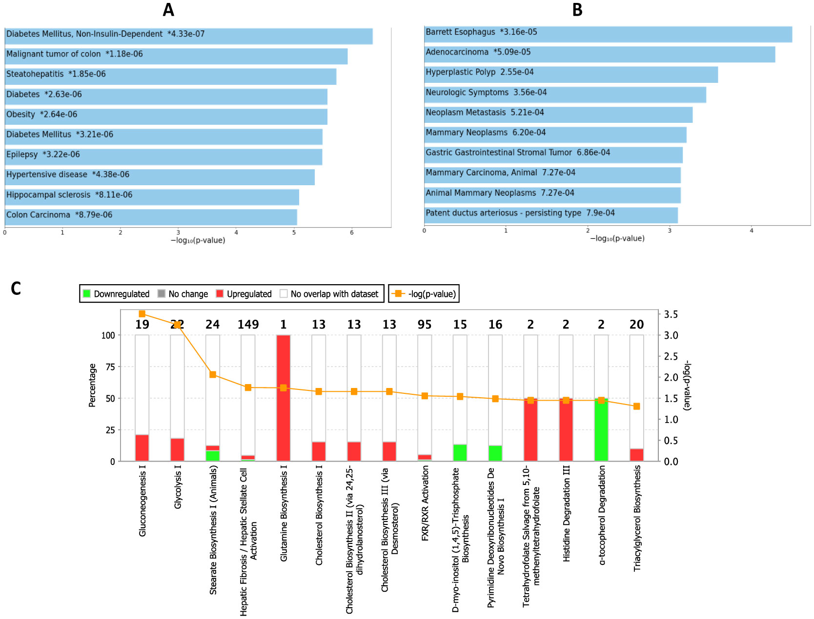
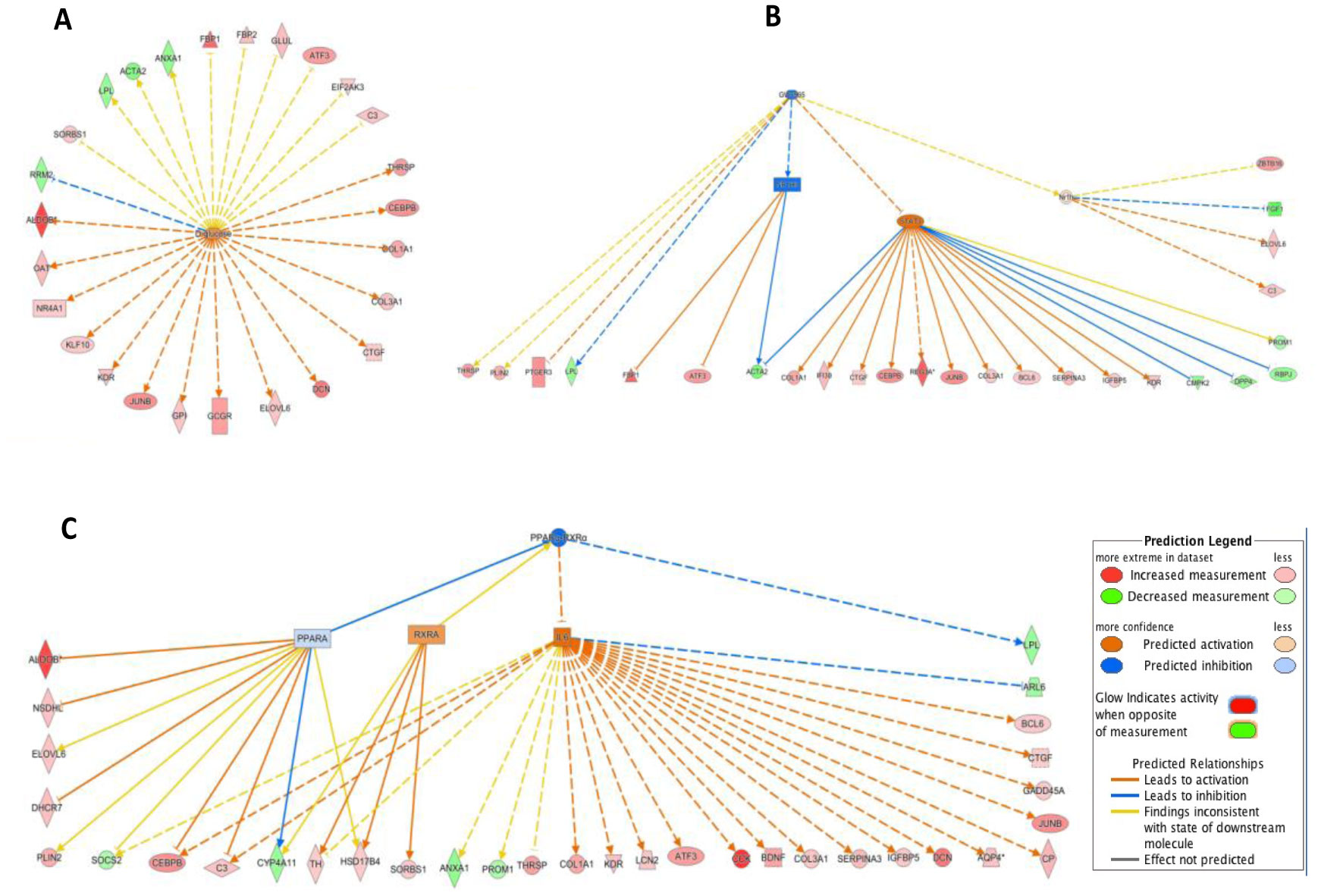
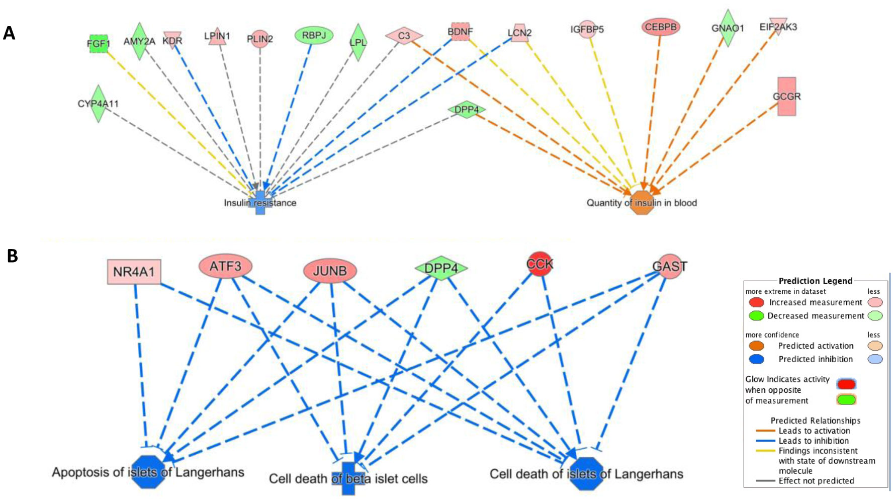
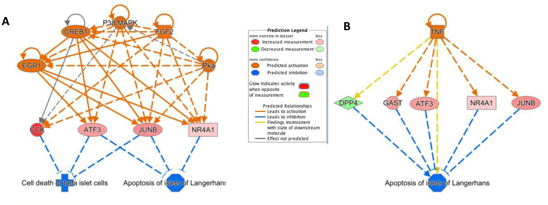
Type 2 diabetes (T2D) is a major global health problem often caused by the inability of pancreatic islets to compensate for the high insulin demand due to apoptosis. However, the complex mechanisms underlying the activation of apoptosis and its counter process, anti-apoptosis, during T2D remain unclear. In this study, we employed bioinformatics and systems biology approaches to understand the anti-apoptosis-associated gene expression and the biological network in the pancreatic islets of T2D mice. First, gene expression data from four peripheral tissues (islets, liver, muscle and adipose) were used to identify differentially expressed genes (DEGs) in T2D compared to non-T2D mouse strains. Our comparative analysis revealed that Gm2036 is upregulated across all four tissues in T2D and is functionally associated with increased cytosolic Ca2+ levels, which may alter the signal transduction pathways controlling metabolic processes. Next, our study focused on islets and performed functional enrichment analysis, which revealed that upregulated genes are significantly associated with sucrose and fructose metabolic processes, as well as negative regulation of neuron apoptosis. Using the Ingenuity Pathway Analysis (IPA) tool of QIAGEN, gene regulatory networks and their biological effects were analyzed, which revealed that glucose is associated with the underlying change in gene expression in the islets of T2D; and an activated gene regulatory network—containing upregulated CCK, ATF3, JUNB, NR4A1, GAST and downregulated DPP4—is possibly inhibiting apoptosis of islets and β-cells in T2D. Our computational-based study has identified a putative regulatory network that may facilitate the survival of pancreatic islets in T2D; however, further validation in a larger sample size is needed. Our results provide valuable insights into the underlying mechanisms of T2D and may offer potential targets for developing more efficacious treatments.
Citation: Firoz Ahmed. Deciphering the gene regulatory network associated with anti-apoptosis in the pancreatic islets of type 2 diabetes mice using computational approaches[J]. AIMS Bioengineering, 2023, 10(2): 111-140. doi: 10.3934/bioeng.2023009
Type 2 diabetes (T2D) is a major global health problem often caused by the inability of pancreatic islets to compensate for the high insulin demand due to apoptosis. However, the complex mechanisms underlying the activation of apoptosis and its counter process, anti-apoptosis, during T2D remain unclear. In this study, we employed bioinformatics and systems biology approaches to understand the anti-apoptosis-associated gene expression and the biological network in the pancreatic islets of T2D mice. First, gene expression data from four peripheral tissues (islets, liver, muscle and adipose) were used to identify differentially expressed genes (DEGs) in T2D compared to non-T2D mouse strains. Our comparative analysis revealed that Gm2036 is upregulated across all four tissues in T2D and is functionally associated with increased cytosolic Ca2+ levels, which may alter the signal transduction pathways controlling metabolic processes. Next, our study focused on islets and performed functional enrichment analysis, which revealed that upregulated genes are significantly associated with sucrose and fructose metabolic processes, as well as negative regulation of neuron apoptosis. Using the Ingenuity Pathway Analysis (IPA) tool of QIAGEN, gene regulatory networks and their biological effects were analyzed, which revealed that glucose is associated with the underlying change in gene expression in the islets of T2D; and an activated gene regulatory network—containing upregulated CCK, ATF3, JUNB, NR4A1, GAST and downregulated DPP4—is possibly inhibiting apoptosis of islets and β-cells in T2D. Our computational-based study has identified a putative regulatory network that may facilitate the survival of pancreatic islets in T2D; however, further validation in a larger sample size is needed. Our results provide valuable insights into the underlying mechanisms of T2D and may offer potential targets for developing more efficacious treatments.

| [1] |
Zheng Y, Ley SH, Hu FB (2018) Global aetiology and epidemiology of type 2 diabetes mellitus and its complications. Nat Rev Endocrinol 14: 88-98. https://doi.org/10.1038/nrendo.2017.151 
|
| [2] |
van Dam RM (2003) The epidemiology of lifestyle and risk for type 2 diabetes. Eur J Epidemiol 18: 1115-1125. https://doi.org/10.1023/b:ejep.0000006612.70245.24
|
| [3] |
Shaw JE, Chisholm DJ (2003) 1: Epidemiology and prevention of type 2 diabetes and the metabolic syndrome. Med J Aust 179: 379-383. https://doi.org/10.5694/j.1326-5377.2003.tb05677.x
|
| [4] |
Dendup T, Feng X, Clingan S, et al. (2018) Environmental risk factors for developing type 2 diabetes mellitus: a systematic review. Int J Environ Res Public Health 15: 78. https://doi.org/10.3390/ijerph15010078
|
| [5] | Joseph JS, Anand K, Malindisa ST, et al. (2021) Exercise, CaMKII, and type 2 diabetes. EXCLI J 20: 386-399. https://doi.org/10.17179/excli2020-3317 |
| [6] |
Tanabe K, Liu Y, Hasan SD, et al. (2011) Glucose and fatty acids synergize to promote B-cell apoptosis through activation of glycogen synthase kinase 3β independent of JNK activation. PLoS One 6: e18146. https://doi.org/10.1371/journal.pone.0018146
|
| [7] |
Poitout V, Robertson RP (2008) Glucolipotoxicity: fuel excess and beta-cell dysfunction. Endocr Rev 29: 351-366. https://doi.org/10.1210/er.2007-0023
|
| [8] |
Rutter GA, Chimienti F (2015) SLC30A8 mutations in type 2 diabetes. Diabetologia 58: 31-36. https://doi.org/10.1007/s00125-014-3405-7
|
| [9] |
Al-Sinani S, Woodhouse N, Al-Mamari A, et al. (2015) Association of gene variants with susceptibility to type 2 diabetes among Omanis. World J Diabetes 6: 358-366. https://doi.org/10.4239/wjd.v6.i2.358
|
| [10] |
Prasad RB, Groop L (2015) Genetics of type 2 diabetes-pitfalls and possibilities. Genes 6: 87-123. https://doi.org/10.3390/genes6010087
|
| [11] |
Xue A, Wu Y, Zhu Z, et al. (2018) Genome-wide association analyses identify 143 risk variants and putative regulatory mechanisms for type 2 diabetes. Nat Commun 9: 2941. https://doi.org/10.1038/s41467-018-04951-w
|
| [12] |
Röder PV, Wu B, Liu Y, et al. (2016) Pancreatic regulation of glucose homeostasis. Exp Mol Med 48: e219. https://doi.org/10.1038/emm.2016.6
|
| [13] |
Dolenšek J, Rupnik MS, Stožer A (2015) Structural similarities and differences between the human and the mouse pancreas. Islets 7: e1024405. https://doi.org/10.1080/19382014.2015.1024405
|
| [14] |
Campbell JE, Newgard CB (2021) Mechanisms controlling pancreatic islet cell function in insulin secretion. Nat Rev Mol Cell Biol 22: 142-158. https://doi.org/10.1038/s41580-020-00317-7
|
| [15] |
Lan H, Rabaglia ME, Stoehr JP, et al. (2003) Gene expression profiles of nondiabetic and diabetic obese mice suggest a role of hepatic lipogenic capacity in diabetes susceptibility. Diabetes 52: 688-700. https://doi.org/10.2337/diabetes.52.3.688
|
| [16] | da Silva Rosa SC, Nayak N, Caymo AM, et al. (2020) Mechanisms of muscle insulin resistance and the cross-talk with liver and adipose tissue. Physiol Rep 8: e14607. https://doi.org/10.14814/phy2.14607 |
| [17] |
Donath MY, Ehses JA, Maedler K, et al. (2005) Mechanisms of beta-cell death in type 2 diabetes. Diabetes 54: S108-S113. https://doi.org/10.2337/diabetes.54.suppl_2.s108
|
| [18] |
Chang-Chen KJ, Mullur R, Bernal-Mizrachi E (2008) Beta-cell failure as a complication of diabetes. Rev Endocr Metab Disord 9: 329-343. https://doi.org/10.1007/s11154-008-9101-5
|
| [19] |
Rahier J, Guiot Y, Goebbels RM, et al. (2008) Pancreatic beta-cell mass in European subjects with type 2 diabetes. Diabetes Obes Metab 10: 32-42. https://doi.org/10.1111/j.1463-1326.2008.00969.x
|
| [20] |
Butler AE, Janson J, Bonner-Weir S, et al. (2003) Beta-cell deficit and increased beta-cell apoptosis in humans with type 2 diabetes. Diabetes 52: 102-110. https://doi.org/10.2337/diabetes.52.1.102
|
| [21] |
Butler AE, Janson J, Soeller WC, et al. (2003) Increased beta-cell apoptosis prevents adaptive increase in beta-cell mass in mouse model of type 2 diabetes: evidence for role of islet amyloid formation rather than direct action of amyloid. Diabetes 52: 2304-2314. https://doi.org/10.2337/diabetes.52.9.2304
|
| [22] |
Rhodes CJ (2005) Type 2 diabetes-a matter of beta-cell life and death?. Science 307: 380-384. https://doi.org/10.1126/science.1104345
|
| [23] |
Araujo TG, Oliveira AG, Saad MJ (2013) Insulin-resistance-associated compensatory mechanisms of pancreatic Beta cells: a current opinion. Front Endocrinol (Lausanne) 4: 146. https://doi.org/10.3389/fendo.2013.00146
|
| [24] |
Migliorini A, Bader E, Lickert H (2014) Islet cell plasticity and regeneration. Mol Metab 3: 268-274. https://doi.org/10.1016/j.molmet.2014.01.010
|
| [25] |
Johnson JD, Yang YHC, Luciani DS (2015) Mechanisms of pancreatic β-cell apoptosis in diabetes and its therapies. Islets of Langerhans . Netherlands: Springer 873-894.
|
| [26] |
Tomita T (2010) Immunocytochemical localisation of caspase-3 in pancreatic islets from type 2 diabetic subjects. Pathology 42: 432-437. https://doi.org/10.3109/00313025.2010.493863
|
| [27] |
Tomita T (2016) Apoptosis in pancreatic beta-islet cells in Type 2 diabetes. Bosn J Basic Med Sci 16: 162-179. https://doi.org/10.17305/bjbms.2016.919
|
| [28] |
Ho FM, Liu SH, Liau CS, et al. (2000) High glucose-induced apoptosis in human endothelial cells is mediated by sequential activations of c-Jun NH(2)-terminal kinase and caspase-3. Circulation 101: 2618-2624. https://doi.org/10.1161/01.CIR.101.22.2618
|
| [29] |
Federici M, Hribal M, Perego L, et al. (2001) High glucose causes apoptosis in cultured human pancreatic islets of Langerhans: a potential role for regulation of specific Bcl family genes toward an apoptotic cell death program. Diabetes 50: 1290-1301. https://doi.org/10.2337/diabetes.50.6.1290
|
| [30] |
Johnson JD, Luciani DS (2010) Mechanisms of pancreatic beta-cell apoptosis in diabetes and its therapies. Adv Exp Med Biol 654: 447-462. https://doi.org/10.1007/978-90-481-3271-3_19
|
| [31] |
Talchai C, Xuan S, Lin HV, et al. (2012) Pancreatic beta cell dedifferentiation as a mechanism of diabetic beta cell failure. Cell 150: 1223-1234. https://doi.org/10.1016/j.cell.2012.07.029
|
| [32] |
Avrahami D, Wang YJ, Schug J, et al. (2020) Single-cell transcriptomics of human islet ontogeny defines the molecular basis of β-cell dedifferentiation in T2D. Mol Metab 42: 101057. https://doi.org/10.1016/j.molmet.2020.101057
|
| [33] |
Efanova IB, Zaitsev SV, Zhivotovsky B, et al. (1998) Glucose and tolbutamide induce apoptosis in pancreatic beta-cells. A process dependent on intracellular Ca2+ concentration. J Biol Chem 273: 33501-33507. https://doi.org/10.1074/jbc.273.50.33501
|
| [34] |
Lickert H (2013) Betatrophin fuels beta cell proliferation: first step toward regenerative therapy?. Cell Metab 18: 5-6. https://doi.org/10.1016/j.cmet.2013.06.006
|
| [35] |
Crunkhorn S (2013) Metabolic disorders: betatrophin boosts beta-cells. Nat Rev Drug Discov 12: 504. https://doi.org/10.1038/nrd4058
|
| [36] |
Kugelberg E (2013) Diabetes: Betatrophin--inducing beta-cell expansion to treat diabetes mellitus?. Nat Rev Endocrinol 9: 379. https://doi.org/10.1038/nrendo.2013.98
|
| [37] |
Laing E, Smith CP (2010) RankProdIt: A web-interactive rank products analysis tool. BMC Res Notes 3: 221. https://doi.org/10.1186/1756-0500-3-221
|
| [38] |
Breitling R, Armengaud P, Amtmann A, et al. (2004) Rank products: a simple, yet powerful, new method to detect differentially regulated genes in replicated microarray experiments. FEBS Lett 573: 83-92. https://doi.org/10.1016/j.febslet.2004.07.055
|
| [39] |
Piñero J, Queralt-Rosinach N, Bravo À, et al. (2015) DisGeNET: a discovery platform for the dynamical exploration of human diseases and their genes. Database 2015: bav028. https://doi.org/10.1093/database/bav028
|
| [40] | Xie Z, Bailey A, Kuleshov MV, et al. (2021) Gene set knowledge discovery with enrichr. Curr Protoc 1: e90. https://doi.org/10.1002/cpz1.90 |
| [41] |
Clarke DJB, Jeon M, Stein DJ, et al. (2021) Appyters: Turning jupyter notebooks into data-driven web apps. Patterns 2: 100213. https://doi.org/10.1016/j.patter.2021.100213
|
| [42] |
Krämer A, Green J, Pollard J, et al. (2014) Causal analysis approaches in Ingenuity Pathway Analysis. Bioinformatics 30: 523-530. https://doi.org/10.1093/bioinformatics/btt703
|
| [43] |
Moreno-Asso A, Castaño C, Grilli A, et al. (2013) Glucose regulation of a cell cycle gene module is selectively lost in mouse pancreatic islets during ageing. Diabetologia 56: 1761-1772. https://doi.org/10.1007/s00125-013-2930-0
|
| [44] |
Anderson DM, Makarewich CA, Anderson KM, et al. (2016) Widespread control of calcium signaling by a family of SERCA-inhibiting micropeptides. Sci Signal 9: ra119. https://doi.org/10.1126/scisignal.aaj1460
|
| [45] |
Rossi AE, Dirksen RT (2006) Sarcoplasmic reticulum: the dynamic calcium governor of muscle. Muscle Nerve 33: 715-731. https://doi.org/10.1002/mus.20512
|
| [46] |
Sabatini PV, Speckmann T, Lynn FC (2019) Friend and foe: β-cell Ca. Mol Metab 21: 1-12. https://doi.org/10.1016/j.molmet.2018.12.007
|
| [47] |
Srinivasan S, Bernal-Mizrachi E, Ohsugi M, et al. (2002) Glucose promotes pancreatic islet beta-cell survival through a PI 3-kinase/Akt-signaling pathway. Am J Physiol Endocrinol Metab 283: E784-E793. https://doi.org/10.1152/ajpendo.00177.2002
|
| [48] |
Klec C, Ziomek G, Pichler M, et al. (2019) Calcium signaling in ß-cell physiology and pathology: a revisit. Int J Mol Sci 20: 6110. https://doi.org/10.3390/ijms20246110
|
| [49] |
Li K, Jiang Y, Xiang X, et al. (2020) Long non-coding RNA SNHG6 promotes the growth and invasion of non-small cell lung cancer by downregulating miR-101-3p. Thorac Cancer 11: 1180-1190. https://doi.org/10.1111/1759-7714.13371
|
| [50] | Meng Q, Zhang F, Chen H, et al. lncRNA SNHG6 improves placental villous cell function in an in vitro model of gestational diabetes mellitus (2020). https://doi.org/10.5114/aoms.2020.100643 |
| [51] |
Xu Z, Zuo Y, Wang J, et al. (2015) Overexpression of the regulator of G-protein signaling 5 reduces the survival rate and enhances the radiation response of human lung cancer cells. Oncol Rep 33: 2899-2907. https://doi.org/10.3892/or.2015.3917
|
| [52] |
Deng W, Wang X, Xiao J, et al. (2012) Loss of regulator of G protein signaling 5 exacerbates obesity, hepatic steatosis, inflammation and insulin resistance. PLoS One 7: e30256. https://doi.org/10.1371/journal.pone.0030256
|
| [53] |
Sun Y, Gao HY, Fan ZY, et al. (2020) Metabolomics signatures in type 2 diabetes: A systematic review and integrative analysis. J Clin Endocrinol Metab 105: 1000-1008. https://doi.org/10.1210/clinem/dgz240
|
| [54] |
Ahmed F, Khan AA, Ansari HR, et al. (2022) A systems biology and LASSO-based approach to decipher the transcriptome-interactome signature for predicting non-small cell lung cancer. Biology 11: 1752. https://doi.org/10.3390/biology11121752
|
| [55] |
Ahmed F (2020) A network-based analysis reveals the mechanism underlying vitamin D in suppressing cytokine storm and virus in SARS-CoV-2 infection. Front Immunol 11: 590459. https://doi.org/10.3389/fimmu.2020.590459
|
| [56] |
Ahmed F (2019) Integrated network analysis reveals FOXM1 and MYBL2 as key regulators of cell proliferation in non-small cell lung cancer. Front Oncol 9: 1011. https://doi.org/10.3389/fonc.2019.01011
|
| [57] |
Marselli L, Thorne J, Dahiya S, et al. (2010) Gene expression profiles of Beta-cell enriched tissue obtained by laser capture microdissection from subjects with type 2 diabetes. PLoS One 5: e11499. https://doi.org/10.1371/journal.pone.0011499
|
| [58] |
Ostenson CG, Khan A, Abdel-Halim SM, et al. (1993) Abnormal insulin secretion and glucose metabolism in pancreatic islets from the spontaneously diabetic GK rat. Diabetologia 36: 3-8. https://doi.org/10.1007/BF00399086
|
| [59] |
Khan A, Chandramouli V, Ostenson CG, et al. (1990) Glucose cycling in islets from healthy and diabetic rats. Diabetes 39: 456-459. https://doi.org/10.2337/diab.39.4.456
|
| [60] |
Thomas HE, McKenzie MD, Angstetra E, et al. (2009) Beta cell apoptosis in diabetes. Apoptosis 14: 1389-1404. https://doi.org/10.1007/s10495-009-0339-5
|
| [61] |
Costes S, Bertrand G, Ravier MA (2021) Mechanisms of beta-cell apoptosis in type 2 diabetes-prone situations and potential protection by GLP-1-based therapies. Int J Mol Sci 22: 5303. https://doi.org/10.3390/ijms22105303
|
| [62] |
Šrámek J, Němcová-Fürstová V, Kovář J (2021) Molecular mechanisms of apoptosis induction and its regulation by fatty acids in pancreatic β-cells. Int J Mol Sci 22: 4285. https://doi.org/10.3390/ijms22084285
|
| [63] |
Shen S, Wang F, Fernandez A, et al. (2020) Role of platelet-derived growth factor in type II diabetes mellitus and its complications. Diab Vasc Dis Res 17: 1479164120942119. https://doi.org/10.1177/1479164120942119
|
| [64] |
Shan Z, Xu C, Wang W, et al. (2019) Enhanced PDGF signaling in gestational diabetes mellitus is involved in pancreatic β-cell dysfunction. Biochem Biophys Res Commun 516: 402-407. https://doi.org/10.1016/j.bbrc.2019.06.048
|
| [65] |
Qin JJ, Yan L, Zhang J, et al. (2019) STAT3 as a potential therapeutic target in triple negative breast cancer: a systematic review. J Exp Clin Cancer Res 38: 195. https://doi.org/10.1186/s13046-019-1206-z
|
| [66] |
Jiang M, Li B (2022) STAT3 and its targeting inhibitors in oral squamous cell carcinoma. Cells 11: 3131. https://doi.org/10.3390/cells11193131
|
| [67] |
Gorogawa S, Fujitani Y, Kaneto H, et al. (2004) Insulin secretory defects and impaired islet architecture in pancreatic beta-cell-specific STAT3 knockout mice. Biochem Biophys Res Commun 319: 1159-1170. https://doi.org/10.1016/j.bbrc.2004.05.095
|
| [68] |
Weng Q, Zhao M, Zheng J, et al. (2020) STAT3 dictates β-cell apoptosis by modulating PTEN in streptozocin-induced hyperglycemia. Cell Death Differ 27: 130-145. https://doi.org/10.1038/s41418-019-0344-3
|
| [69] |
Kisseleva T, Bhattacharya S, Braunstein J, et al. (2002) Signaling through the JAK/STAT pathway, recent advances and future challenges. Gene 285: 1-24. https://doi.org/10.1016/s0378-1119(02)00398-0
|
| [70] |
Zong CS, Chan J, Levy DE, et al. (2000) Mechanism of STAT3 activation by insulin-like growth factor I receptor. J Biol Chem 275: 15099-15105. https://doi.org/10.1074/jbc.M000089200
|
| [71] |
De Groef S, Renmans D, Cai Y, et al. (2016) STAT3 modulates β-cell cycling in injured mouse pancreas and protects against DNA damage. Cell Death Dis 7: e2272. https://doi.org/10.1038/cddis.2016.171
|
| [72] |
Dalle S, Quoyer J, Varin E, et al. (2011) Roles and regulation of the transcription factor CREB in pancreatic β-cells. Curr Mol Pharmacol 4: 187-195. https://doi.org/10.2174/1874467211104030187
|
| [73] |
Krabbe KS, Nielsen AR, Krogh-Madsen R, et al. (2007) Brain-derived neurotrophic factor (BDNF) and type 2 diabetes. Diabetologia 50: 431-438. https://doi.org/10.1007/s00125-006-0537-4
|
| [74] |
Sun K, Wernstedt Asterholm I, Kusminski CM, et al. (2012) Dichotomous effects of VEGF-A on adipose tissue dysfunction. Proc Natl Acad Sci USA 109: 5874-5879. https://doi.org/10.1073/pnas.1200447109
|
| [75] |
Guo H, Jin D, Zhang Y, et al. (2010) Lipocalin-2 deficiency impairs thermogenesis and potentiates diet-induced insulin resistance in mice. Diabetes 59: 1376-1385. https://doi.org/10.2337/db09-1735
|
| [76] |
Pajvani UB, Shawber CJ, Samuel VT, et al. (2011) Inhibition of notch signaling ameliorates insulin resistance in a FoxO1-dependent manner. Nat Med 17: 961-967. https://doi.org/10.1038/nm.2378
|
| [77] |
Liu S, Croniger C, Arizmendi C, et al. (1999) Hypoglycemia and impaired hepatic glucose production in mice with a deletion of the C/EBPbeta gene. J Clin Invest 103: 207-213. https://doi.org/10.1172/JCI4243
|
| [78] |
Greenbaum LE, Li W, Cressman DE, et al. (1998) CCAAT enhancer-binding protein beta is required for normal hepatocyte proliferation in mice after partial hepatectomy. J Clin Invest 102: 996-1007. https://doi.org/10.1172/JCI3135
|
| [79] |
Wang L, Shao J, Muhlenkamp P, et al. (2000) Increased insulin receptor substrate-1 and enhanced skeletal muscle insulin sensitivity in mice lacking CCAAT/enhancer-binding protein beta. J Biol Chem 275: 14173-14181. https://doi.org/10.1074/jbc.m000764200
|
| [80] |
Lavine JA, Raess PW, Stapleton DS, et al. (2010) Cholecystokinin is up-regulated in obese mouse islets and expands beta-cell mass by increasing beta-cell survival. Endocrinology 151: 3577-3588. https://doi.org/10.1210/en.2010-0233
|
| [81] |
Meek TH, Wisse BE, Thaler JP, et al. (2013) BDNF action in the brain attenuates diabetic hyperglycemia via insulin-independent inhibition of hepatic glucose production. Diabetes 62: 1512-1518. https://doi.org/10.2337/db12-0837
|
| [82] |
Mattson MP, Maudsley S, Martin B (2004) BDNF and 5-HT: a dynamic duo in age-related neuronal plasticity and neurodegenerative disorders. Trends Neurosci 27: 589-594. https://doi.org/10.1016/j.tins.2004.08.001
|
| [83] |
Mattson MP (2007) Calcium and neurodegeneration. Aging Cell 6: 337-350. https://doi.org/10.1111/j.1474-9726.2007.00275.x
|
| [84] |
Harding HP, Zeng H, Zhang Y, et al. (2001) Diabetes mellitus and exocrine pancreatic dysfunction in perk-/- mice reveals a role for translational control in secretory cell survival. Mol Cell 7: 1153-1163. https://doi.org/10.1016/s1097-2765(01)00264-7
|
| [85] |
Zhang P, McGrath B, Li S, et al. (2002) The PERK eukaryotic initiation factor 2 alpha kinase is required for the development of the skeletal system, postnatal growth, and the function and viability of the pancreas. Mol Cell Biol 22: 3864-3874. https://doi.org/10.1128/mcb.22.11.3864-3874.2002
|
| [86] |
Cavener DR, Gupta S, McGrath BC (2010) PERK in beta cell biology and insulin biogenesis. Trends Endocrinol Metab 21: 714-721. https://doi.org/10.1016/j.tem.2010.08.005
|
| [87] |
Gurzov EN, Barthson J, Marhfour I, et al. (2012) Pancreatic beta-cells activate a JunB/ATF3-dependent survival pathway during inflammation. Oncogene 31: 1723-1732. https://doi.org/10.1038/onc.2011.353
|
| [88] |
Tellez N, Joanny G, Escoriza J, et al. (2011) Gastrin treatment stimulates beta-cell regeneration and improves glucose tolerance in 95% pancreatectomized rats. Endocrinology 152: 2580-2588. https://doi.org/10.1210/en.2011-0066
|
| [89] |
Yu C, Cui S, Zong C, et al. (2015) The orphan nuclear receptor NR4A1 protects pancreatic beta-cells from endoplasmic reticulum (ER) stress-mediated apoptosis. J Biol Chem 290: 20687-20699. https://doi.org/10.1074/jbc.M115.654863
|
| [90] | Ogura A, Nishida T, Hayashi Y, et al. (1991) The development of the uteroplacental vascular system in the golden hamster mesocricetus auratus. J Anat 175: 65-77. |
| [91] |
Ruest LB, Marcotte R, Wang E (2002) Peptide elongation factor eEF1A-2/S1 expression in cultured differentiated myotubes and its protective effect against caspase-3-mediated apoptosis. J Biol Chem 277: 5418-5425. https://doi.org/10.1074/jbc.M110685200
|
| [92] |
Sun Y, Du C, Wang B, et al. (2014) Up-regulation of eEF1A2 promotes proliferation and inhibits apoptosis in prostate cancer. Biochem Biophys Res Commun 450: 1-6. https://doi.org/10.1016/j.bbrc.2014.05.045
|
| [93] |
Larsson LI, Rehfeld JF, Sundler F, et al. (1976) Pancreatic gastrin in foetal and neonatal rats. Nature 262: 609-610. https://doi.org/10.1038/262609a0
|
| [94] |
Povoski SP, Zhou W, Longnecker DS, et al. (1994) Stimulation of in vivo pancreatic growth in the rat is mediated specifically by way of cholecystokinin-A receptors. Gastroenterology 107: 1135-1146. https://doi.org/10.1016/0016-5085(94)90239-9
|
| [95] |
Röhrborn D, Wronkowitz N, Eckel J (2015) DPP4 in diabetes. Front Immunol 6: 386. https://doi.org/10.3389/fimmu.2015.00386
|
| [96] |
Boer GA, Holst JJ (2020) Incretin Hormones and Type 2 Diabetes-Mechanistic Insights and Therapeutic Approaches. Biology 9: 473. https://doi.org/10.3390/biology9120473
|
| [97] |
Nagamine A, Hasegawa H, Hashimoto N, et al. (2017) The effects of DPP-4 inhibitor on hypoxia-induced apoptosis in human umbilical vein endothelial cells. J Pharmacol Sci 133: 42-48. https://doi.org/10.1016/j.jphs.2016.12.003
|
| [98] |
Sato K, Aytac U, Yamochi T, et al. (2003) CD26/dipeptidyl peptidase IV enhances expression of topoisomerase II alpha and sensitivity to apoptosis induced by topoisomerase II inhibitors. Br J Cancer 89: 1366-1374. https://doi.org/10.1038/sj.bjc.6601253
|
| [99] | Pro B, Dang NH (2004) CD26/dipeptidyl peptidase IV and its role in cancer. Histol Histopathol 19: 1345-1351. https://doi.org/10.14670/HH-19.1345 |
| [100] |
Gaetaniello L, Fiore M, de Filippo S, et al. (1998) Occupancy of dipeptidyl peptidase IV activates an associated tyrosine kinase and triggers an apoptotic signal in human hepatocarcinoma cells. Hepatology 27: 934-942. https://doi.org/10.1002/hep.510270407
|
| [101] |
Huang CN, Wang CJ, Lee YJ, et al. (2017) Active subfractions of abelmoschus esculentus substantially prevent free fatty acid-induced β cell apoptosis via inhibiting dipeptidyl peptidase-4. PLoS One 12: e0180285. https://doi.org/10.1371/journal.pone.0180285
|
| [102] |
Kim W, Egan JM (2008) The role of incretins in glucose homeostasis and diabetes treatment. Pharmacol Rev 60: 470-512. https://doi.org/10.1124/pr.108.000604
|
| [103] |
Kim SJ, Winter K, Nian C, et al. (2005) Glucose-dependent insulinotropic polypeptide (GIP) stimulation of pancreatic beta-cell survival is dependent upon phosphatidylinositol 3-kinase (PI3K)/protein kinase B (PKB) signaling, inactivation of the forkhead transcription factor Foxo1, and down-regulation of bax expression. J Biol Chem 280: 22297-22307. https://doi.org/10.1074/jbc.M500540200
|
| [104] |
Ehses JA, Casilla VR, Doty T, et al. (2003) Glucose-dependent insulinotropic polypeptide promotes beta-(INS-1) cell survival via cyclic adenosine monophosphate-mediated caspase-3 inhibition and regulation of p38 mitogen-activated protein kinase. Endocrinology 144: 4433-4445. https://doi.org/10.1210/en.2002-0068
|
| [105] |
Farngren J, Persson M, Ahren B (2018) Effects on the glucagon response to hypoglycaemia during DPP-4 inhibition in elderly subjects with type 2 diabetes: A randomized, placebo-controlled study. Diabetes Obes Metab 20: 1911-1920. https://doi.org/10.1111/dom.13316
|
| [106] |
Senmaru T, Fukui M, Kobayashi K, et al. (2012) Dipeptidyl-peptidase IV inhibitor is effective in patients with type 2 diabetes with high serum eicosapentaenoic acid concentrations. J Diabetes Investig 3: 498-502. https://doi.org/10.1111/j.2040-1124.2012.00220.x
|
| [107] |
Kim YG, Hahn S, Oh TJ, et al. (2013) Differences in the glucose-lowering efficacy of dipeptidyl peptidase-4 inhibitors between Asians and non-Asians: a systematic review and meta-analysis. Diabetologia 56: 696-708. https://doi.org/10.1007/s00125-012-2827-3
|
| [108] |
Park H, Park C, Kim Y, et al. (2012) Efficacy and safety of dipeptidyl peptidase-4 inhibitors in type 2 diabetes: meta-analysis. Ann Pharmacother 46: 1453-1469. https://doi.org/10.1345/aph.1R041
|
| [109] |
Panina G (2007) The DPP-4 inhibitor vildagliptin: robust glycaemic control in type 2 diabetes and beyond. Diabetes Obes Metab 9: 32-39. https://doi.org/10.1111/j.1463-1326.2007.00763.x
|
 bioeng-10-02-009-s001.zip bioeng-10-02-009-s001.zip |
 |
Figures(6) / Tables(4)

Firoz Ahmed. Deciphering the gene regulatory network associated with anti-apoptosis in the pancreatic islets of type 2 diabetes mice using computational approaches[J]. AIMS Bioengineering, 2023, 10(2): 111-140. doi: 10.3934/bioeng.2023009


 DownLoad: