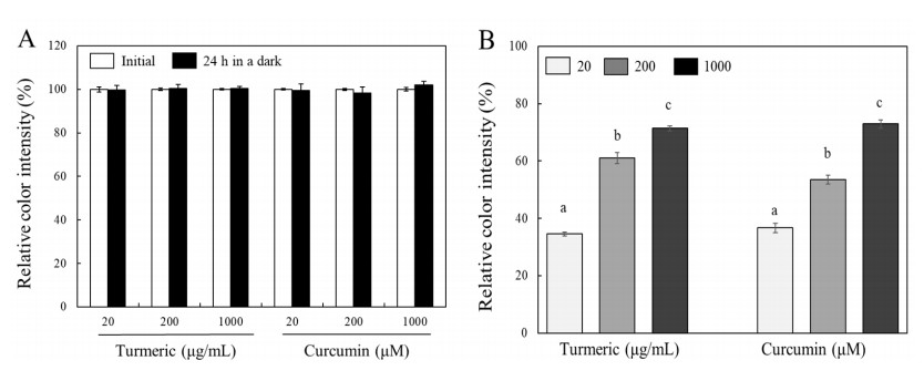
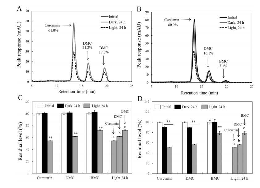
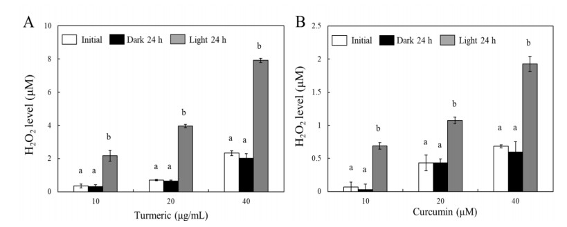
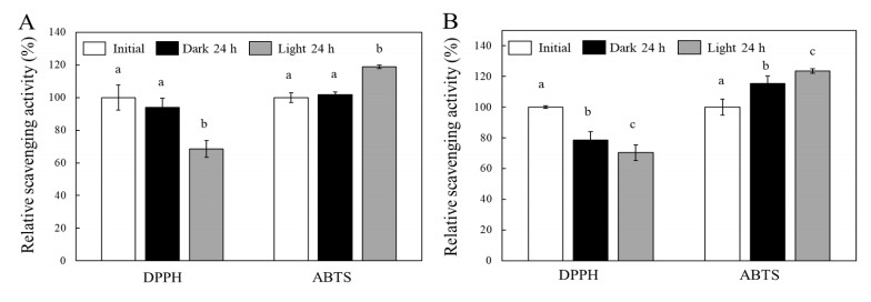
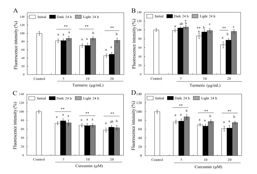
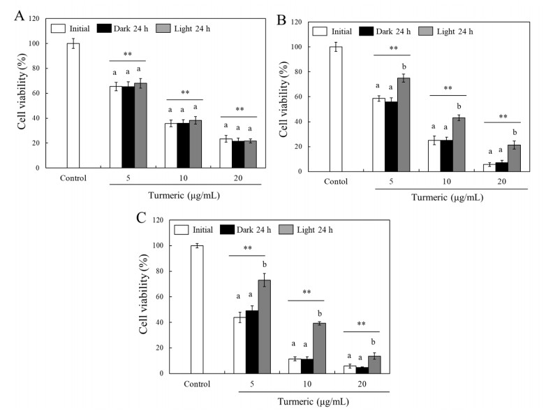
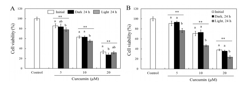
Turmeric pigments have attracted a great attention for their variety of physiological functions. The pigments are, however, chemically unstable under various conditions including light irradiation. In this study, changes in chemical characteristics and bioactivities of turmeric pigments under light were investigated. Chemical changes of turmeric oleoresin (20 µg/mL) and curcumin (20 μM) significantly proceeded under irradiation by a regular household fluorescent light (27 W, 30 cm distance). After 24 h irradiation, color intensity of turmeric and curcumin decreased by 65.4 and 63.0%, respectively. Among three curcuminoids in turmeric, bisdemethoxycurcumin was the most resistant to decomposition by light. Scavenging activities of the irradiated turmeric pigments against 2, 2-diphenyl-2-picrylhydrazyl radical and intracellular reactive oxygen species were significantly less pronounced. The activity against 2'-azino-bis-(3-ethylbenzothiazoline-6-sulfonic acid radical was, however, significantly enhanced after photo-degradation. Cytotoxic effects of turmeric oleoresin after 24 h irradiation on HCT 116 colon cancer cells decreased, while those of curcumin was enhanced after photo-degradation. Our results indicates that chemical properties and bioactivities of turmeric pigments can be modulated under light, and the phenomena should be considered in various processing and storage conditions for the pigment-containing foods.
Citation: Yu Na Jung, Jungil Hong. Changes in chemical properties and bioactivities of turmeric pigments by photo-degradation[J]. AIMS Agriculture and Food, 2021, 6(2): 754-767. doi: 10.3934/agrfood.2021045
Turmeric pigments have attracted a great attention for their variety of physiological functions. The pigments are, however, chemically unstable under various conditions including light irradiation. In this study, changes in chemical characteristics and bioactivities of turmeric pigments under light were investigated. Chemical changes of turmeric oleoresin (20 µg/mL) and curcumin (20 μM) significantly proceeded under irradiation by a regular household fluorescent light (27 W, 30 cm distance). After 24 h irradiation, color intensity of turmeric and curcumin decreased by 65.4 and 63.0%, respectively. Among three curcuminoids in turmeric, bisdemethoxycurcumin was the most resistant to decomposition by light. Scavenging activities of the irradiated turmeric pigments against 2, 2-diphenyl-2-picrylhydrazyl radical and intracellular reactive oxygen species were significantly less pronounced. The activity against 2'-azino-bis-(3-ethylbenzothiazoline-6-sulfonic acid radical was, however, significantly enhanced after photo-degradation. Cytotoxic effects of turmeric oleoresin after 24 h irradiation on HCT 116 colon cancer cells decreased, while those of curcumin was enhanced after photo-degradation. Our results indicates that chemical properties and bioactivities of turmeric pigments can be modulated under light, and the phenomena should be considered in various processing and storage conditions for the pigment-containing foods.

| [1] | Delgado-Vargas F, Paredes-López O (2002) Natural colorants for food and nutraceutical uses, In: Chapter 4, Pigments as Food Colorants, Boca Raton: CRC Press, 35-59. |
| [2] | Yasaei PM, Yang GC, Warner CR, et al. (1996) Singlet oxygen oxidation of lipids resulting from photochemical sensitizers in the presence of antioxidants. J Am Soc 73: 1177-1181. |
| [3] |
Min D, Boff J (2002) Chemistry and reaction of singlet oxygen in foods. Compr Rev Food Sci Food Saf 1: 58-72. doi: 10.1111/j.1541-4337.2002.tb00007.x

|
| [4] |
Kotra VSR, Satyabanta L, Goswami TK (2019) A critical review of analytical methods for determination of curcuminoids in turmeric. J Food Sci Technol 56: 5153-5166. doi: 10.1007/s13197-019-03986-1
|
| [5] | Ahmad RS, Hussain MB, Sultan MT, et al. (2020) Biochemistry, safety, pharmacological activities, and clinical applications of turmeric: A mechanistic review. Evid Based Complement Alternat Med 10: 7656919. |
| [6] |
Amalraj A, Pius A, Gopi S, et al. (2016) Biological activities of curcuminoids, other biomolecules from turmeric and their derivatives-A review. J Tradit Complement Med 7: 205-233. doi: 10.1016/j.jtcme.2016.05.005
|
| [7] |
Memarzia A, Khazdair MR, Behrouz S, et al. (2021) Experimental and clinical reports on anti-inflammatory, antioxidant, and immunomodulatory effects of Curcuma longa and curcumin, an updated and comprehensive review. Biofactors 47: 311-350. doi: 10.1002/biof.1716
|
| [8] |
Zheng D, Huang C, Huang H, et al. (2020) Antibacterial mechanism of curcumin: A review. Chem Biodivers 17: e2000171. doi: 10.1002/cbdv.202000171
|
| [9] |
Bhat A, Mahalakshmi AM, Ray B, et al. (2019) Benefits of curcumin in brain disorders. Biofactors 45: 666-689. doi: 10.1002/biof.1533
|
| [10] |
Kunnumakkara AB, Bordoloi D, Harsha C, et al. (2017) Curcumin mediates anticancer effects by modulating multiple cell signaling pathways. Clin Sci (Lond) 131:1781-1799. doi: 10.1042/CS20160935
|
| [11] |
Li L, Zhang X, Pi C, et al. (2020) Review of curcumin physicochemical targeting delivery system. Int J Nanomedicine 15: 9799-9821. doi: 10.2147/IJN.S276201
|
| [12] |
Priyadarsini KI (2009) Photophysics, Photochemistry and photobiology of curcumin: studies from organic solutions, bio-mimetics and living cells. J Photochem Photobiol C: Photochem Rev 10: 81-95. doi: 10.1016/j.jphotochemrev.2009.05.001
|
| [13] |
Nardo L, Andreoni A, Masson M, et al. (2011) Studies on curcumin and curcuminoids. XXXIX. Photophysical properties of bisdemethoxycurcumin. J Fluoresc 21: 627-635. doi: 10.1007/s10895-010-0750-x
|
| [14] |
Lee BH, Choi HA, Kim M, et al. (2013) Changes in chemical stability and bioactivities of curcumin by ultraviolet radiation. Food Sci Biotechnol 22: 279-282. doi: 10.1007/s10068-013-0038-4
|
| [15] |
Jiang ZY, Woollard ACS, Wolff SP (1991) Lipid hydroperoxide measurement by oxidation of Fe2+ in the presence of xylenol orange. Comparison with the TBA assay and an iodometric method. Lipids 26: 853-856. doi: 10.1007/BF02536169
|
| [16] |
Blois MS. (1958) Antioxidant determination by the use of a stable free radical. Nature 26: 1199-1203. doi: 10.1038/1811199a0
|
| [17] |
Jara PJ, Fulgencio SC (2006) Effect of solvent and certain food constituents on different antioxidant capacity assays. Food Res Int 39: 791-800. doi: 10.1016/j.foodres.2006.02.003
|
| [18] |
LeBel CP, Ischiropoulos H, Bondy SC. (1992) Evaluation of the probe 2', 7'-dichlorofluorescin as an indicator of reactive oxygen species formation and oxidative Stress. Chem Res Toxicol 5: 227-231. doi: 10.1021/tx00026a012
|
| [19] |
Dearden J, Forbes W (1960) The Study of hydrogen bonding and related phenomena by ultraviolet light absorption: Part Iv. Intermolecular hydrogen bonding in anilines and phenols. Can J Chem 38: 896-910. doi: 10.1139/v60-127
|
| [20] |
Schneider C, Gordon ON, Edwards RL, et al. (2015) Degradation of curcumin: from mechanism to biological implications. J Agric Food Chem 63: 7606-7614. doi: 10.1021/acs.jafc.5b00244
|
| [21] |
Gordon ON, Luis PB, Ashley RE, et al. (2015) Oxidative transformation of demethoxy-and bisdemethoxycurcumin: products, mechanism of formation, and poisoning of human topoisomerase Ⅱα. Chem Res Toxicol 28: 989-996. doi: 10.1021/acs.chemrestox.5b00009
|
| [22] |
Saitawee D, Teerakapong A, Morales NP, et al. (2018) Photodynamic therapy of Curcuma longa extract stimulated with blue light against Aggregatibacter actinomycetemcomitans. Photodiagnosis Photodyn Ther 22: 101-105. doi: 10.1016/j.pdpdt.2018.03.001
|
| [23] |
Ak T, Gülçin İ (2008) Antioxidant and radical scavenging properties of curcumin. Chem Biol Interact 174: 27-37. doi: 10.1016/j.cbi.2008.05.003
|
| [24] |
Wang Y, Pan M, Cheng A, et al. (1997) Stability of curcumin in buffer solutions and characterization of its degradation products. J Pharm Biomed Anal 15: 1867-1876. doi: 10.1016/S0731-7085(96)02024-9
|
| [25] |
Shen L, Ji H (2012) The Pharmacology of curcumin: Is it the degradation products? Trends Mol Med 18: 138-144. doi: 10.1016/j.molmed.2012.01.004
|
| [26] |
Jung YN, Kang S, Lee BH et al. (2016) Changes in the chemical properties and anti-oxidant activities of curcumin by microwave radiation. Food Sci Biotechnol 25: 1449-1455. doi: 10.1007/s10068-016-0225-1
|
| [27] | Song E, Kang S, Hong J (2018) Changes in chemical properties, antioxidant activities, and cytotoxicity of turmeric pigments by thermal process. Korean J Food Sci Technol 50: 21-27. |
| [28] |
Apel K, Hirt H (2004) Reactive oxygen species: metabolism, oxidative stress, and signal transduction. Annu Rev Plant Biol 55: 373-399. doi: 10.1146/annurev.arplant.55.031903.141701
|
| [29] |
Cerutti PA (1985) Prooxidant states and tumor promotion. science 227: 375-381. doi: 10.1126/science.2981433
|
| [30] |
Klaunig JE, Kamendulis LM (2004) The role of oxidative stress in a carcinogenesis. Annu Rev Pharmacol Toxicol 44: 239-267. doi: 10.1146/annurev.pharmtox.44.101802.121851
|
| [31] |
Daniel S, Limson JL, Dairam A, et al. (2004) Through metal binding, curcumin protects against lead-and cadmium-induced lipid peroxidation in rat brain homogenates and against lead-induced tissue damage in rat brain. J Inorg Biochem 98: 266-275. doi: 10.1016/j.jinorgbio.2003.10.014
|
| [32] |
Barzegar A, Moosavi-Movahedi AA (2011) Intracellular ROS protection efficiency and free radical-scavenging activity of curcumin. PLoS One. 6: e26012. doi: 10.1371/journal.pone.0026012
|
| [33] |
Mortezaee K, Salehi E, Mirtavoos-Mahyari H, et al. (2019) Mechanisms of apoptosis modulation by curcumin: Implications for cancer therapy. J Cell Physiol 234: 12537-12550. doi: 10.1002/jcp.28122
|
| [34] | Hong J. (2007) Curcumin-Induced Growth Inhibitory effects on HeLa Cells altered by antioxidant modulators. Food Sci Biotechnol 16: 1029-1034. |
| [35] | Heo Y, Hong J (2020) Changes in chemical stability and biological activities of sinapinic acid by heat treatment under different pH conditions. Korean J Food Sci Technol 52: 616-621. |
Figures(7)

Yu Na Jung, Jungil Hong. Changes in chemical properties and bioactivities of turmeric pigments by photo-degradation[J]. AIMS Agriculture and Food, 2021, 6(2): 754-767. doi: 10.3934/agrfood.2021045


 DownLoad: