Accurate computation of Greeks for equity-linked security (ELS) near early redemption dates

Yunjae Nam; Changwoo Yoo; Hyundong Kim; Jaewon Hong; Minjoon Bang; Junseok Kim; Yunjae Nam; Changwoo Yoo; Hyundong Kim; Jaewon Hong; Minjoon Bang; Junseok Kim

doi:10.3934/QFE.2025010

Quantitative Finance and Economics

2025, Volume 9, Issue 2: 300-316. doi: 10.3934/QFE.2025010

Previous Article Next Article

Research article

Accurate computation of Greeks for equity-linked security (ELS) near early redemption dates

1.
Program in Actuarial Science and Financial Engineering, Korea University, Seoul 02841, Republic of Korea
2.
Department of Mathematics and Physics, Gangneung-Wonju National University, Gangneung 25457, Republic of Korea
3.
Department of Mathematics, Korea University, Seoul 02841, Republic of Korea

Received: 14 January 2025 Revised: 17 March 2025 Accepted: 21 April 2025 Published: 24 April 2025
JEL Codes: C63, G13, G12

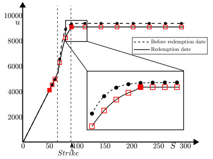
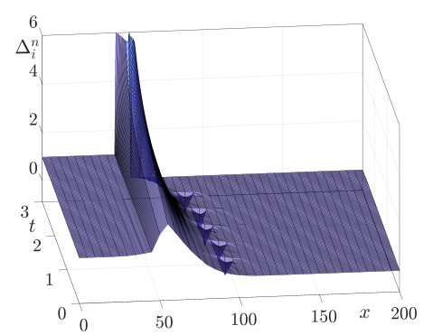
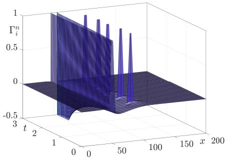
This study presents a numerical method for accurately computing the option values and Greeks of equity-linked securities (ELS) near early redemption dates. The Black–Scholes (BS) equation is solved using the finite difference method (FDM), and a Dirichlet boundary condition is applied at strike prices instead of directly replacing option values above the strike price with predefined option prices. This approach improves the accuracy of option pricing, particularly in the presence of early redemption structures. The proposed method is demonstrated to be effective in computing Greeks, which are crucial for risk management and hedging strategies in ELS markets. The computational tests validate the reliability of the method in capturing the sensitivities of ELS prices to various market factors.
- Equity-linked securities,
- Greeks,
- Finite difference method
Citation: Yunjae Nam, Changwoo Yoo, Hyundong Kim, Jaewon Hong, Minjoon Bang, Junseok Kim. Accurate computation of Greeks for equity-linked security (ELS) near early redemption dates[J]. Quantitative Finance and Economics, 2025, 9(2): 300-316. doi: 10.3934/QFE.2025010

Related Papers:

Abstract

This study presents a numerical method for accurately computing the option values and Greeks of equity-linked securities (ELS) near early redemption dates. The Black–Scholes (BS) equation is solved using the finite difference method (FDM), and a Dirichlet boundary condition is applied at strike prices instead of directly replacing option values above the strike price with predefined option prices. This approach improves the accuracy of option pricing, particularly in the presence of early redemption structures. The proposed method is demonstrated to be effective in computing Greeks, which are crucial for risk management and hedging strategies in ELS markets. The computational tests validate the reliability of the method in capturing the sensitivities of ELS prices to various market factors.

References

[1]	Anderson D, Ulrych U (2023) Accelerated American option pricing with deep neural networks. Quant Financ Econ 7: 207–228. https://doi.org/10.3934/QFE.2023011 doi: 10.3934/QFE.2023011
[2]	Black F, Scholes M (1973) The pricing of options and corporate liabilities. J Polit Econ 81: 637–654. https://doi.org/10.1086/260062 doi: 10.1086/260062
[3]	Cui Y, Li L, Zhang G (2024) Pricing and hedging autocallable products by Markov chain approximation. Rev Deriv Res 27: 1–45.
[4]	Hwang Y, Kim I, Kwak S, et al. (2023) Unconditionally stable monte carlo simulation for solving the multi-dimensional Allen–Cahn equation. Electron Res Arch 31. https://doi.org/10.3934/era.2023261 doi: 10.3934/era.2023261
[5]	Jo J, Kim Y (2013) Comparison of numerical schemes on multi-dimensional Black–Scholes equations. Bull Korean Math Soc 50: 2035–2051. https://doi.org/10.4134/BKMS.2013.50.6.2035 doi: 10.4134/BKMS.2013.50.6.2035
[6]	Kanamura T (2018) Diversification effect of commodity futures on financial markets. Quant Financ Econ 2: 821–836. https://doi.org/10.3934/QFE.2018.4.821 doi: 10.3934/QFE.2018.4.821
[7]	Kim ST, Kim HG, Kim JH (2021) ELS pricing and hedging in a fractional Brownian motion environment. Chaos Solitons Fractals 142: 110453. https://doi.org/10.1016/j.chaos.2020.110453 doi: 10.1016/j.chaos.2020.110453
[8]	Kwak S, Kang S, Ham S, et al. (2023) An unconditionally stable difference scheme for the two‐dimensional modified Fisher–Kolmogorov–Petrovsky–Piscounov equation. J Math 2023: 5527728. https://doi.org/10.1155/2023/5527728 doi: 10.1155/2023/5527728
[9]	Larguinho M, Dias JC, Braumann CA (2022) Pricing and hedging bond options and sinking-fund bonds under the CIR model. Quant Financ Econ 6: 1–34. https://doi.org/10.3934/QFE.2022001 doi: 10.3934/QFE.2022001
[10]	Lee H, Ha H, Kong B, et al. (2024) Valuing three-asset barrier options and autocallable products via exit probabilities of Brownian bridge. N Am Econ Financ 73: 102174. https://doi.org/10.1016/j.najef.2024.102174 doi: 10.1016/j.najef.2024.102174
[11]	Lee C, Kwak S, Hwang Y, et al. (2023) Accurate and efficient finite difference method for the Black–Scholes model with no far-field boundary conditions. Comput Econ 61: 1207–1224. https://doi.org/10.1007/s10614-022-10242-w doi: 10.1007/s10614-022-10242-w
[12]	Liu T, Li T, Ullah MZ (2024) On five-point equidistant stencils based on Gaussian function with application in numerical multi-dimensional option pricing. Comput Math Appl 176: 35–45. https://doi.org/10.1016/j.camwa.2024.09.003 doi: 10.1016/j.camwa.2024.09.003
[13]	Liu T, Soleymani F, Ullah MZ (2024) Solving multi-dimensional European option pricing problems by integrals of the inverse quadratic radial basis function on non-uniform meshes. Chaos Solitons Fractals 185: 115156. https://doi.org/10.1016/j.chaos.2024.115156 doi: 10.1016/j.chaos.2024.115156
[14]	Lyu J, Park E, Kim S, et al. (2021) Optimal non-uniform finite difference grids for the Black–Scholes equations. Math Comput Simul 182: 690–704. https://doi.org/10.1016/j.matcom.2020.12.002 doi: 10.1016/j.matcom.2020.12.002
[15]	Roul P, Goura VP (2020) A sixth order numerical method and its convergence for generalized Black–Scholes PDE. J Comput Appl Math 377: 112881. https://doi.org/10.1016/j.cam.2020.112881 doi: 10.1016/j.cam.2020.112881
[16]	Tao L, Lai Y, Ji Y, et al. (2023) Asian option pricing under sub-fractional Vasicek model. Quant Finan Econ 7: 403–419. https://doi.org/10.3934/QFE.2023020 doi: 10.3934/QFE.2023020
[17]	Thomas Thomas L (1949) Elliptic Problems in Linear Differential Equations Over a Network: Watson Scientific Computing Laboratory. Columbia University: New York, NY, USA
[18]	Wang Y, Yan K (2023) Machine learning-based quantitative trading strategies across different time intervals in the American market. Quant Financ Econ 7: 569–594. https://doi.org/10.3934/QFE.2023028 doi: 10.3934/QFE.2023028
[19]	Wu X, Wen S, Shao W, et al. (2023) Numerical Investigation of Fractional Step-Down ELS Option. Fractal Fract 7: 126. https://doi.org/10.3390/fractalfract7020126 doi: 10.3390/fractalfract7020126

Reader Comments

Your name:*

Email:*
© 2025 the Author(s), licensee AIMS Press. This is an open access article distributed under the terms of the Creative Commons Attribution License (http://creativecommons.org/licenses/by/4.0)