Plasma HGF concentration in patients with brain tumors

Zygmunt Siedlecki; Sebastian Grzyb; Danuta Rość; Maciej Śniegocki; Zygmunt Siedlecki; Sebastian Grzyb; Danuta Rość; Maciej Śniegocki

doi:10.3934/Neuroscience.2020008

AIMS Neuroscience

2020, Volume 7, Issue 2: 107-119. doi: 10.3934/Neuroscience.2020008

Previous Article Next Article

Research article

Plasma HGF concentration in patients with brain tumors

Running title:Running headline: HGF in patients with brain tumors

1.
Department of Neurosurgery and Neurotraumatology and Pediatric Neurosurgery, Collegium Medicum in Bydgoszcz of Nicolaus Copernicus University in Toruń, Poland
2.
Department of Pathophysiology, Collegium Medicum in Bydgoszcz of Nicolaus Copernicus University in Toruń, Poland

Received: 24 March 2020 Accepted: 21 April 2020 Published: 30 April 2020

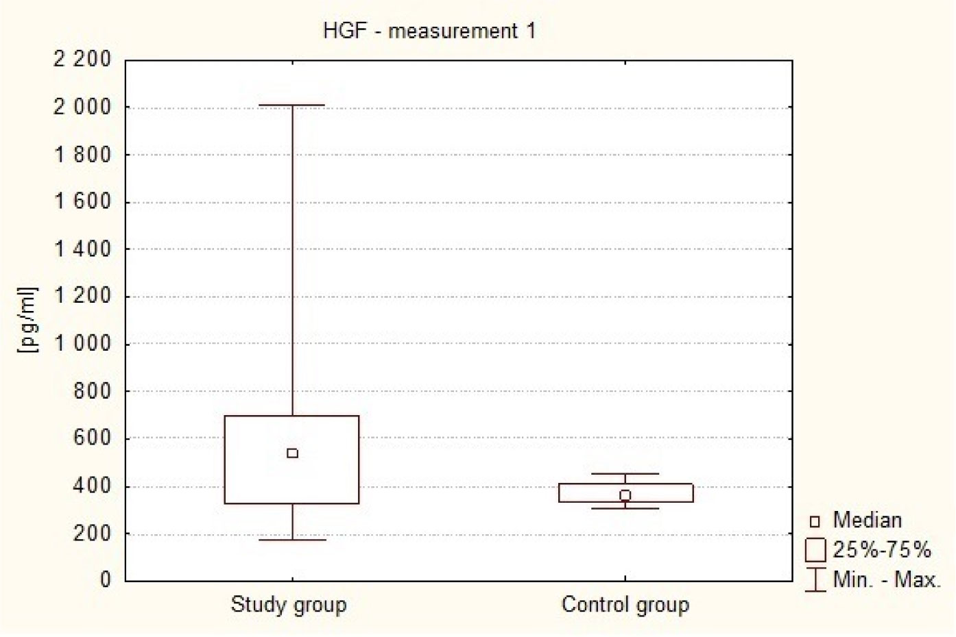
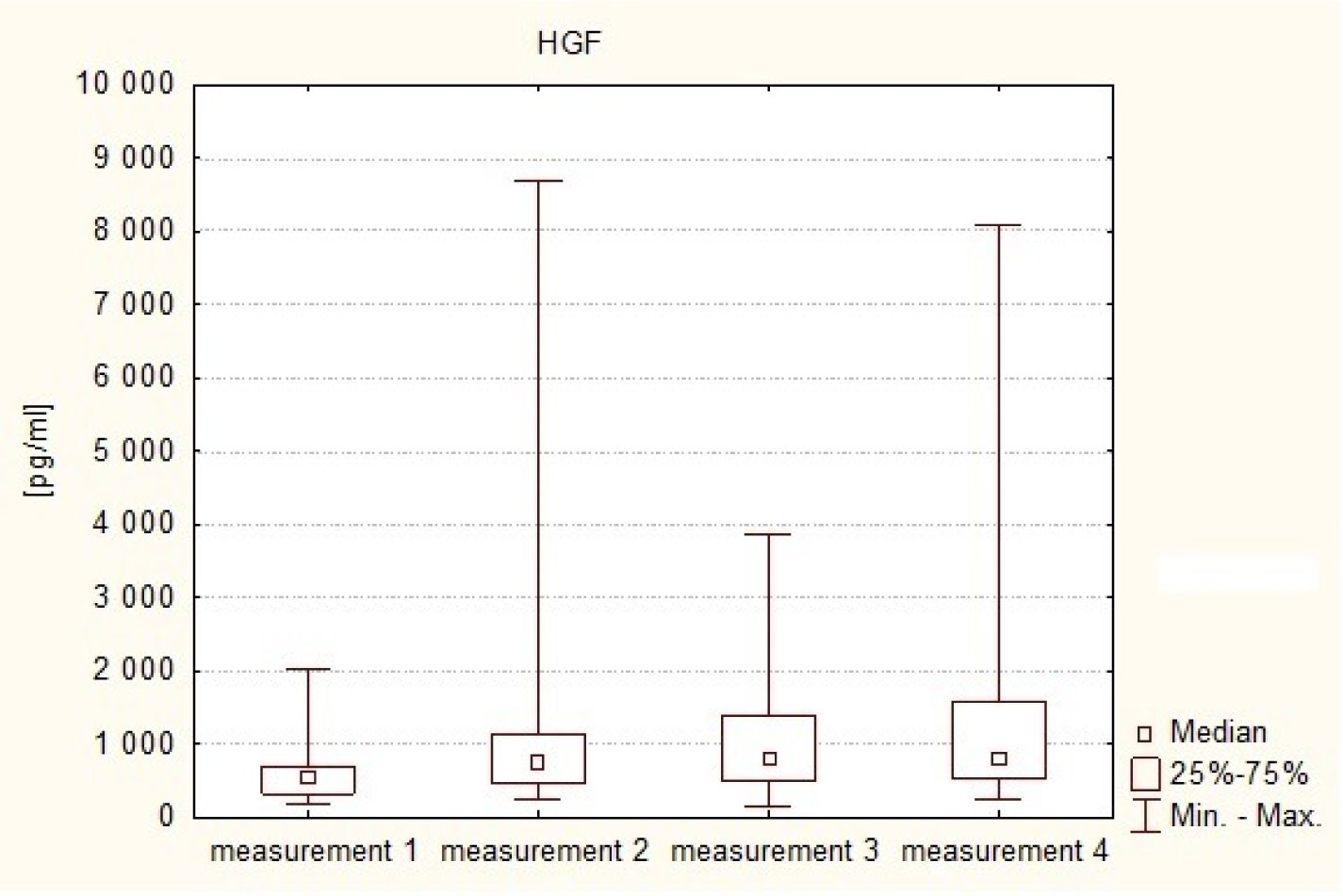
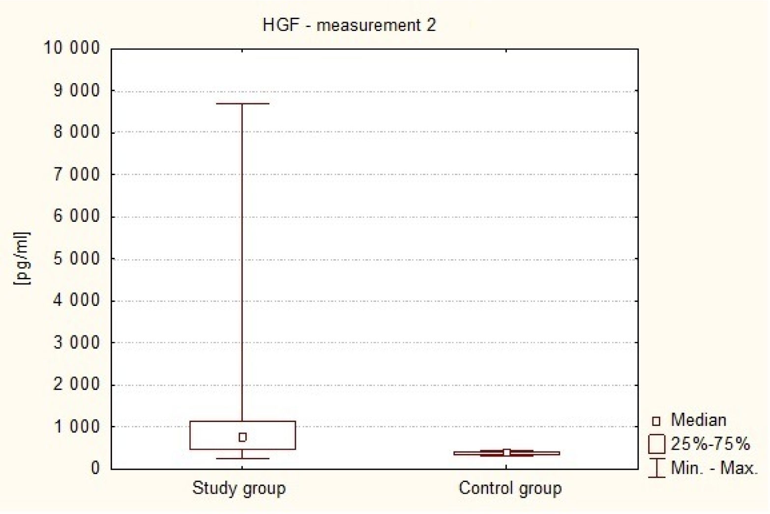
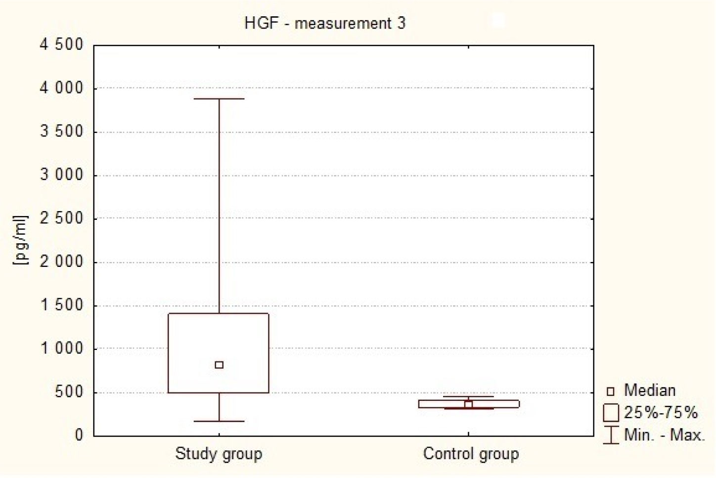
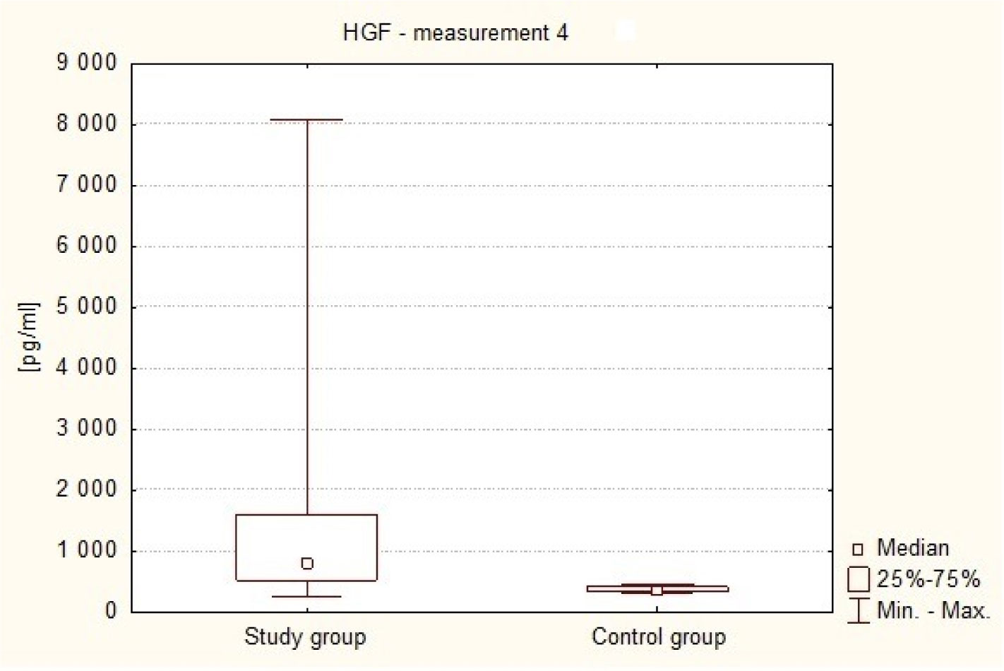
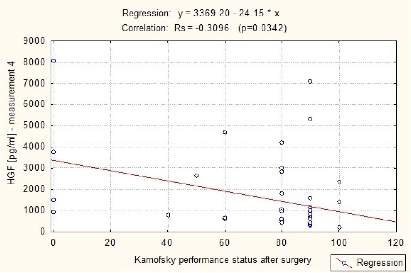
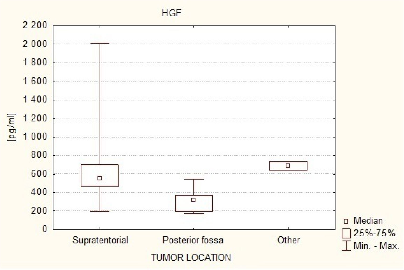
The Hepatocyte Growth Factor is a strong mitogenic factor and seems to play important role in tumor angiogenesis. The purpose of this study was to analyse the plasma concentration of this factor in patients treated surgically because of intracranial tumors. The study included 47 patients, both sexes treated surgically for intracranial tumors and 30 adult volunteers of both sexes, without cancer diagnosis. In study group 4 measurements of plasma HGF were taken: measurement 1: within 24 hours to 1 hour before the operation (preoperative), measurement 2: on the first day after the operation, i.e. after 24 hours, measurement 3: between the third and fifth day following the treatment, i.e. within 72–120 hours, and measurement 4: on the seventh day after the operation, i.e. after 840 hours. In control group only one measurement was taken. The distribution of the analyzed parameters was different from the normal distribution, therefore nonparametric statistics were used. The result values are presented in the form of a median (Me). The analysis revealed that HGR plasma levels in the patients with intracranial tumors in all 4 measurements (Me1 = 543.16 pg/ml, Me2 = 762.59 pg/ml, Me3 = 819.82 pg/ml, Me4 = 804.82 pg/ml) in the perioperative period were elevated in comparison to healthy subjects (Me = 361.04 pg/ml). The association has been shown to exist between postoperative HGF plasma levels and the clinical condition of patients with intracranial tumors (p = 0.0342). Postoperative HGF levels correlated negatively with the patients' postoperative condition. It was also found that in patients with supratentorial tumors HGF plasma levels were higher (Me = 557.74 pg/ml) in comparison to patients with posterior fossa tumors (Me = 325.00 pg/ml). These results suggest increased angiogenic and mitogenic activity in patients with intracranial tumors and its even greater intensity in the postoperative period. Greater angiogenic activity appears to occur in patients with supratentorial tumors.

Keywords:

Citation: Zygmunt Siedlecki, Sebastian Grzyb, Danuta Rość, Maciej Śniegocki. Plasma HGF concentration in patients with brain tumors[J]. AIMS Neuroscience, 2020, 7(2): 107-119. doi: 10.3934/Neuroscience.2020008

Related Papers:

[1]	D. L. Suthar, D. Baleanu, S. D. Purohit, F. Uçar . Certain k-fractional calculus operators and image formulas of k-Struve function. AIMS Mathematics, 2020, 5(3): 1706-1719. doi: 10.3934/math.2020115
[2]	Shahid Mubeen, Rana Safdar Ali, Iqra Nayab, Gauhar Rahman, Thabet Abdeljawad, Kottakkaran Sooppy Nisar . Integral transforms of an extended generalized multi-index Bessel function. AIMS Mathematics, 2020, 5(6): 7531-7547. doi: 10.3934/math.2020482
[3]	Gauhar Rahman, Shahid Mubeen, Kottakkaran Sooppy Nisar . On generalized $\mathtt{k}$ -fractional derivative operator. AIMS Mathematics, 2020, 5(3): 1936-1945. doi: 10.3934/math.2020129
[4]	Saima Naheed, Shahid Mubeen, Gauhar Rahman, M. R. Alharthi, Kottakkaran Sooppy Nisar . Some new inequalities for the generalized Fox-Wright functions. AIMS Mathematics, 2021, 6(6): 5452-5464. doi: 10.3934/math.2021322
[5]	Khaled Mehrez, Abdulaziz Alenazi . Bounds for certain function related to the incomplete Fox-Wright function. AIMS Mathematics, 2024, 9(7): 19070-19088. doi: 10.3934/math.2024929
[6]	Sabila Ali, Shahid Mubeen, Rana Safdar Ali, Gauhar Rahman, Ahmed Morsy, Kottakkaran Sooppy Nisar, Sunil Dutt Purohit, M. Zakarya . Dynamical significance of generalized fractional integral inequalities via convexity. AIMS Mathematics, 2021, 6(9): 9705-9730. doi: 10.3934/math.2021565
[7]	Muajebah Hidan, Mohamed Akel, Hala Abd-Elmageed, Mohamed Abdalla . Solution of fractional kinetic equations involving extended $(k, \tau)$ -Gauss hypergeometric matrix functions. AIMS Mathematics, 2022, 7(8): 14474-14491. doi: 10.3934/math.2022798
[8]	D. L. Suthar, A. M. Khan, A. Alaria, S. D. Purohit, J. Singh . Extended Bessel-Maitland function and its properties pertaining to integral transforms and fractional calculus. AIMS Mathematics, 2020, 5(2): 1400-1410. doi: 10.3934/math.2020096
[9]	Ji Hyang Park, Hari Mohan Srivastava, Nak Eun Cho . Univalence and convexity conditions for certain integral operators associated with the Lommel function of the first kind. AIMS Mathematics, 2021, 6(10): 11380-11402. doi: 10.3934/math.2021660
[10]	Kanagaraj Muthuselvan, Baskar Sundaravadivoo, Suliman Alsaeed, Kottakkaran Sooppy Nisar . New interpretation of topological degree method of Hilfer fractional neutral functional integro-differential equation with nonlocal condition. AIMS Mathematics, 2023, 8(7): 17154-17170. doi: 10.3934/math.2023876

Abstract

1. Introduction and preliminaries

Fractional calculus is an essential research area, which is equally useful not only in pure mathematics but also in applied mathematics, physics, biology, engineering, economics and control theory etc. In recent years, study on fractional differential equations is very dynamic and widespread around the world. Some of its applications in diverse fields are discussed in ^[1,2]. Optical solitons of time-fractional higher-order nonlinear Schr $\ddot{o}$ dinger equation and soliton molecule solutions of nonlinear Schr $\ddot{o}$ dinger equations are established by Dai et al. ^[3,4]. A hybrid analytical solution to examine the fractional model of the nonlinear wave-like equation is explored by Kumar et al. ^[5]. Numerical solutions with linearization techniques of the fractional Harry Dym equation are established in ^[6].

Many researchers have discussed fractional calculus operators ^[7,8]. The composition of Erdélyi-Kober fractional operators is presented in ^[9]. Mishra et al. discussed the Marichev-Saigo-Maeda fractional calculus operators on the product of Srivastava polynomials and generalized Mittag-Leffler function ^[10]. Certain Integral operators involving the Gauss hypergeometric functions are elaborated in ^[11,12]. A brief study of fractional calculus operators on generalized multivariable Mittag-Leffler function is presented by Suthar et al. ^[13]. A brief systematic history of the generalized fractional calculus operators and their applications is being profoundly analyzed in ^[14,15]. A concise description of generalized fractional calculus operators together with their applications is available in ^[16,17,18].

A variety of research publications are continuously in progress regarding the generalization of classical fractional calculus operators. In this continuation, many researchers established generalized fractional operator and their applications^[19,20]. Smraiz et al. modified the $(k, s)$ fractional integral operator involving $k$ -Mittag-Leffler function and also discussed the applications of $(k, s)$ -Hilfer-Prabhakar fractional derivative in mathematical physics ^[21,22]. Can et al. have discussed the global existence for a mild solution of fractional Volterra integro-differential equations ^[23] and inverse source problem for the time-fractional diffusion equation with Mittag-Leffler kernel ^[24]. They also explored regularized solution approximation for the fractional pseudo-parabolic problem with a nonlinear source term in ^[25].

For our study, we start with $k$ versions of Saigo fractional integral and derivative operators involving the $k$ -hypergeometric function in the kernel which were introduced by Gupta and Parihar ^[26] and are defined as follows:

For $w\in\mathbb{R^{+}}$ , $\epsilon, \varrho, \chi\in\mathbb{C}$ with $Re(\epsilon) > 0$ , $k > 0$ , we have

$\begin{eqnarray} (I_{0+,k}^{\epsilon,\varrho,\chi}f)(w) = \frac{w^{\frac{-\epsilon-\varrho}{k}}}{k\Gamma_{k}(\epsilon)}\int_{0}^{w}(w-t)^{\frac{\epsilon}{k}-1} \\ \times _{2}F_{1,k}((\epsilon+\varrho,k),(-\chi,k);(\epsilon,k);(1-\frac{t}{w}))f(t)dt. \end{eqnarray}$

(1.1)

$\begin{eqnarray} (I_{-,k}^{\epsilon,\varrho,\chi}f)(w) = \frac{1}{k\Gamma_{k}(\epsilon)}\int_{w}^{\infty}(t-w)^{\frac{\epsilon}{k}-1}t^{\frac{-\epsilon-\varrho}{k}} \\ \times _{2}F_{1,k}((\epsilon+\varrho,k),(-\chi,k);(\epsilon,k);(1-\frac{w}{t}))f(t)dt. \end{eqnarray}$

(1.2)

$\begin{eqnarray} &(D_{0+,k}^{\epsilon,\varrho,\chi}f)(w) = (\frac{d}{dw})^{n}(I_{0+,k}^{-\epsilon+n,-\varrho-n,\epsilon+\chi-n}f)w,\; \; n = [Re(\epsilon)+1] \\ & = (\frac{d}{dw})^{n}\frac{w^{\frac{\epsilon+\varrho}{k}}}{k\Gamma_{k}(-\epsilon+n)}\int_{0}^{w}(w-t)^{\frac{-\epsilon}{k}+n-1} \\ &\times _{2}F_{1,k}((-\epsilon-\varrho,k),(-\chi-\epsilon+n,k);(-\epsilon+n,k);(1-\frac{t}{w}))f(t)dt. \end{eqnarray}$

(1.3)

$\begin{eqnarray} &(D_{-,k}^{\epsilon,\varrho,\chi}f)(w) = (\frac{d}{dw})^{n}(I_{-,k}^{-\epsilon+n,-\varrho-n,\epsilon+\chi}f)w,\; \; n = [Re(\epsilon)+1] \\ & = (\frac{d}{dw})^{n}\frac{1}{k\Gamma_{k}(-\epsilon+n)}\int_{w}^{\infty}(t-w)^{\frac{-\epsilon-n}{k}-1}t^{\frac{\epsilon+\varrho}{k}} \\ &\times _{2}F_{1,k}((-\epsilon-\varrho,k),(-\chi-\epsilon+n,k);(-\epsilon+n,k);(1-\frac{w}{t}))f(t)dt. \end{eqnarray}$

(1.4)

Where $[Re(\epsilon)]$ is the integer part of $Re(\epsilon)$ and $_{2}F_{1, k}((\epsilon, k), (\varrho, k);(\chi, k);w)$ is the $k$ -hypergeometric function defined by Mubeen and Habibullah in ^[19] as:

For $w\in\mathbb{C}$ , $|w| < 1$ , $Re(\chi) > Re(\varrho) > 0$ ,

$\begin{equation} _{2}F_{1,k}((\epsilon,k),(\varrho,k);(\chi,k);w) = \sum\limits_{n = 0}^{\infty}\frac{(\epsilon)_{n,k}(\varrho)_{n,k}w^{n}}{(\chi)_{n,k}n!}. \end{equation}$

(1.5)

The benefit of the generalized $k$ -fractional calculus operators is that they generalize classical Saigo's fractional operators and classical Riemann-Liouville operators. For $k\rightarrow 1$ , (1.1)–(1.4) condense to the Saigo's fractional integral and differential operators ^[11]. If we take $\varrho = -\epsilon$ in (1.1)–(1.4), we have the $k$ - Riemann-Liouville operators as follows:

$\begin{eqnarray} (I_{0+,k}^{\epsilon,\varrho,\chi}f)(w) = (I_{0+,k}^{\epsilon}f)(w), \end{eqnarray}$

(1.6)

$\begin{eqnarray} (I_{-,k}^{\epsilon,\varrho,\chi}f)(w) = (I_{-,k}^{\epsilon}f)(w), \end{eqnarray}$

(1.7)

$\begin{eqnarray} (D_{0+,k}^{\epsilon,\varrho,\chi}f)(w) = (D_{0+,k}^{\epsilon}f)(w), \end{eqnarray}$

(1.8)

$\begin{eqnarray} (D_{-,k}^{\epsilon,\varrho,\chi}f)(w) = (D_{-,k}^{\epsilon}f)(w) \end{eqnarray}$

(1.9)

and for $k\rightarrow 1$ , Eqs (1.6)–(1.9) reduce to classical Riemann-Liouville fractional operators.

Now, we will state the lemmas presented in ^[26] which will be helpful to prove our main results.

Lemma 1.1. Let $\epsilon, \rho, \chi, \lambda\in\mathbb{C}$ , $k\in\mathbb{R}^{+}(0, \infty)$ , $Re(\lambda) > \max[0, Re(\varrho-\chi)]$ . Then

$\begin{equation} (I_{0+,k}^{\epsilon,\varrho,\chi}t^{\frac{\lambda}{k}-1})(w) = \sum\limits_{n = 0}^{\infty}k^{n}\frac{\Gamma_{k}(\lambda)\Gamma_{k}(\lambda-\varrho+\chi)} {\Gamma_{k}(\lambda-\varrho)\Gamma_{k}(\lambda+\epsilon+\chi)}w^{\frac{\lambda-\varrho}{k}-1}. \end{equation}$

(1.10)

Lemma 1.2. Let $\epsilon, \rho, \chi, \lambda\in\mathbb{C}$ , $k\in\mathbb{R}^{+}(0, \infty)$ , $Re(\lambda) > \max[Re(-\varrho), Re(-\chi)]$ . Then

$\begin{equation} (I_{-,k}^{\epsilon,\varrho,\chi}t^{\frac{-\lambda}{k}})(w) = \sum\limits_{n = 0}^{\infty}k^{n}\frac{\Gamma_{k}(\lambda+\varrho)\Gamma_{k}(\lambda+\chi)} {\Gamma_{k}(\lambda)\Gamma_{k}(\lambda+\epsilon+\varrho+\chi)}w^{\frac{-\lambda-\varrho}{k}}. \end{equation}$

(1.11)

Lemma 1.3. Let $\epsilon, \rho, \chi, \lambda\in\mathbb{C}$ , $k\in\mathbb{R}^{+}(0, \infty)$ , $n = Re[\epsilon]+1$ such that $Re(\lambda) > \max[0, Re(-\epsilon-\varrho-\chi)]$ . Then

$\begin{equation} (D_{0+,k}^{\epsilon,\varrho,\chi}t^{\frac{\lambda}{k}-1})(w) = \sum\limits_{n = 0}^{\infty}\frac{\Gamma_{k}(\lambda)\Gamma_{k}(\lambda+\varrho+\chi+\epsilon)} {\Gamma_{k}(\lambda+\chi)\Gamma_{k}(\lambda+\varrho+n-nk)}w^{\frac{\lambda+\varrho+n}{k}-n-1}. \end{equation}$

(1.12)

Lemma 1.4. Let $\epsilon, \rho, \chi, \lambda\in\mathbb{C}$ , $n = Re[\epsilon]+1$ , $k\in\mathbb{R}^{+}(0, \infty)$ such that $Re(\lambda) > max[Re(-\epsilon-\chi), Re(\varrho-nk+n)]$ . Then

$\begin{equation} (D_{-,k}^{\epsilon,\varrho,\chi}t^{\frac{-\lambda}{k}})(w) = \sum\limits_{n = 0}^{\infty}\frac{\Gamma_{k}(\lambda-\varrho-n+nk)\Gamma_{k}(\lambda+\epsilon+\chi)} {\Gamma_{k}(\lambda)\Gamma_{k}(\lambda-\varrho+\chi)}w^{\frac{-\lambda-\varrho+n}{k}-n}. \end{equation}$

(1.13)

Gehlot and Prajapati in ^[27] defined the $k$ -Wright function as follows:

For $k\in\mathbb{R}^{+}$ , $w, a_{i}, b_{j}\in\mathbb{C}$ , $A_{i}, B_{j}\in\mathbb{R} \; (A_{i}, B_{j})\neq 0$ where $i = 1, 2, ..u; j = 1, 2, ..v$ and $(a_{i} + A_{i}n), (b_{j}+B_{j}n) \in \mathbb{C}\setminus k\mathbb{Z}^{-}$ ,

$\begin{equation} _u\psi^{k}_{v}[(a_{1},A_{1}),..(a_{u},A_{u});(b_{1},B_{1}),..(b_{v},B_{v});z] = \sum\limits^\infty_{n = 0}\frac{\Gamma_{k}(a_{1},nA_{1})..\Gamma_{k}(a_{u},nA_{u})z^{n}}{\Gamma_{k}(b_{1},nB_{1})..\Gamma_{k}(b_{v},nB_{v})n!},\\ \end{equation}$

(1.14)

with convergence condition

$\begin{equation} 1+ \sum\limits_{j = 1}^{u}\frac{B_{j}}{k}- \sum\limits_{i = 1}^{v}\frac{A_{i}}{k} > 0, \end{equation}$

(1.15)

for reasonably bounded values of $|z|$ .

The Lommel-Wright $k$ -function is defined as follows:

$\begin{align} J_{\aleph,\hbar,k}^{\wp,m}(z) = (\frac{z}{2})^\frac{\aleph+2\hbar}{k}\sum^\infty_{n = 0} \frac{(-1)^{n}(\frac{z}{2})^{2n}}{(\Gamma_{k}(\hbar+k+nk))^{m}\Gamma_{k} (\aleph+\hbar+k+n\wp)}, \end{align}$

(1.16)

where $z\in \mathbb{C}|(-\infty, 0], \; \wp > 0, \; m\in \mathbb{N}, \; k\in \mathbb{R}, \; \aleph, \hbar\in \mathbb{C}$ and $\Gamma_{k}(Z)$ is the $k$ -gamma function introduced by Diaz and Pariguan ^[28] given by

$\begin{equation*} \Gamma_{k}(z) = lim_{n\rightarrow \infty}\frac{n! k^{n}(nk)^{\frac{\omega}{k}-1}}{(\omega)_{n,k}}, \end{equation*}$

with $k$ -Pochhammer symbol $(\omega)_{n, k}$ given by

$\begin{equation*} (\omega)_{n,k} = \omega(\omega+k) (\omega+2k) . . . . (\omega+(n-1)k),\; \; x\in \mathbb{C}, k\in \mathbb{R}, n\in \mathbb{N}^{+}. \end{equation*}$

The classical Eulers Gamma function and Gamma $k$ -function are related with following relation

$\begin{equation*} \Gamma_{k}(\omega) = k^{\frac{\omega}{k}-1} \Gamma (\frac{\omega}{k}). \end{equation*}$

The Lommel-Wright $k$ -function can also be expressed in the form of $k$ -Wright function as:

$\begin{align} J_{\aleph,\hbar,k}^{\wp,m}(z) = (\frac{z}{2})^\frac{\aleph+2\hbar}{k}\; _1\psi^{k}_{m+1}[(k,k);\underbrace{(\hbar+k,k)}_{m-times},(\aleph+\hbar+k,\wp);\frac{-z^{2}}{4k}]. \end{align}$

(1.17)

For $m = 1$ in (1.16), we define the generalized Bessel-Maitland $k$ -function as:

$\begin{align} J_{\aleph,\hbar,k}^{\wp}(z) = (\frac{z}{2})^\frac{\aleph+2\hbar}{k}\sum^\infty_{n = 0} \frac{(-1)^{n}(\frac{z}{2})^{2n}}{\Gamma_{k}(\hbar+k+nk)\Gamma_{k} (\aleph+\hbar+k+n\wp)}. \end{align}$

(1.18)

It is observed that for $k = 1$ , generalized Lommel-Wright $k$ -function reduces to generalized Lommel-Wright function as given in ^[29] and for $m = k = 1$ , we get the Bessel-Maitland function presented in ^[29]. It also capitulates connection with the classical Bessel function $J_{\aleph}(z)$ mentioned in ^[30] for $m = \wp = k = 1$ and $\hbar = 0$ .

As various kinds of generalized fractional calculus operators involving different special functions are in consistent development. The papers on certain generalized fractional operators and integral transform ^[31,32,33] serve as inspiration for our presented work. This work backs up the prior results and contributes to the field by making broad generalizations.

The layout of the paper is as follows: In section $2$ , we established the formulas for generalized Saigo fractional integrals involving generalized Lommel-Wright function and some of its cases are also discussed as corollaries. Section $3$ is devoted to developing the generalized Saigo fractional differentiation formulas involving generalized Lommel-Wright function along with its special consequences. In Section $4$ , extended Beta transform is applied to the generalized Lommel-Wright function. The last section contains concluding remarks.

2. Saigo k-fractional integration of Lommel-Wright $k$ -function

In this section, we develop the formulas for Saigo $k$ -fractional integrals (1.1) and (1.2) associated with Lommel-Wright $k$ -function. These results are expressed in terms of $k$ -Wright function.

Theorem 2.1. Let $\epsilon, \varrho, \chi, \lambda, \sigma\in\mathbb{C}$ , $\wp > 0$ , $m\in\mathbb{N}$ , $k\in\mathbb{R}^{+}$ , such that $Re(\epsilon) > 0$ , $Re{\lambda} > \max[0, Re(\varrho-\chi)]$ and $Re(\lambda+\chi-\varrho) > 0$ . If condition given by (1.15) is satisfied and $I_{0+, k}^{\epsilon, \varrho, \chi}$ is the left sided integral operator of the generalized $k$ -fractional integration considering $k$ -hypergeometric function. Then the subsequent formula

$\begin{align} &(I_{0+,k}^{\epsilon,\varrho,\chi}t^{\frac{\lambda}{k}-1}J_{\aleph,\hbar,k}^{\wp,m}(t^{\frac{\sigma}{k}}))(w) = w^{\frac{\sigma(\frac{\aleph+2\hbar}{k})+\lambda-\varrho}{k}-1}(\frac{1}{2})^{(\frac{\aleph+2\hbar}{k})}\\[0.3cm] &\times {}_{3}\psi^{k}_{m+3}\left[\begin{array}{c} (\sigma(\frac{\aleph+2\hbar}{k})+\lambda,2\sigma), (\sigma(\frac{\aleph+2\hbar}{k})+\lambda-\varrho+\chi,2\sigma),(k,k);\\ \underbrace{(\hbar+k,k)}_{m-times},(\aleph+\hbar+k,\wp),(\sigma(\frac{\aleph+2\hbar}{k})+\lambda-\varrho,2\sigma),\\ (\sigma(\frac{\aleph+2\hbar}{k})+\lambda+\epsilon+\varrho+\chi,2\sigma); \end{array}\frac{-w^\frac{2\sigma}{k}}{4}\right] \end{align}$

(2.1)

holds.

Proof. Using Eq (1.16) in the left hand side of Eq (2.1), we get

$\begin{align} = \bigg[I_{0+,k}^{\epsilon,\varrho,\chi}t^{\frac{\lambda}{k}-1}\sum^\infty_{n = 0} \frac{(-1)^{n}}{(\Gamma_{k}(\hbar+k+nk))^{m}\Gamma_{k} (\aleph+\hbar+k+n\wp)}\bigg(\frac{t^{\frac{\sigma}{k}}}{2}\bigg)^{\frac{\aleph+2\hbar}{k}+2n}\bigg](w) \end{align}$

(2.2)

$\begin{align} = \sum^\infty_{n = 0} \frac{(-1)^{n}\frac{1}{2}^{\frac{\aleph+2\hbar}{k}+2n}}{(\Gamma_{k}(\hbar+k+nk))^{m}\Gamma_{k} (\aleph+\hbar+k+n\wp)}\bigg[I_{0+,k}^{\epsilon,\varrho,\chi}\bigg(t^{\frac{\sigma(\frac{\aleph+2\hbar}{k})+\lambda+2\sigma n}{k}-1}\bigg)\bigg](w). \end{align}$

(2.3)

Applying Lemma 1.1, we obtain

$\begin{align} & = w^{\frac{\sigma(\frac{\aleph+2\hbar}{k})+\lambda-\varrho}{k}-1}(\frac{1}{2})^{\frac{\aleph+2\hbar}{k}}\sum^\infty_{n = 0} \frac{1}{(\Gamma_{k}(\hbar+k+nk))^{m}\Gamma_{k} (\aleph+\hbar+k+n\wp)}\\ &\times \frac{\Gamma_{k}(\sigma(\frac{\aleph+2\hbar}{k})+\lambda+2\sigma n)\Gamma_{k}(\sigma(\frac{\aleph+2\hbar}{k})+\lambda-\varrho+\chi+2\sigma n)}{\Gamma_{k}(\sigma(\frac{\aleph+2\hbar}{k})+\lambda-\varrho+2\sigma n)\Gamma_{k}(\sigma(\frac{\aleph+2\hbar}{k})+\lambda+\varrho+\epsilon+\chi+2\sigma n)} \bigg(\frac{-kw^{\frac{2\sigma}{k}}}{4}\bigg)^{n}. \end{align}$

(2.4)

Multiplying and dividing by $\Gamma(n+1)$ and using $\Gamma(n+1) = k^{-n}\Gamma_{k}(nk+k)$ , we get

$\begin{align} & = w^{\frac{\sigma(\frac{\aleph+2\hbar}{k})+\lambda-\varrho}{k}-1}(\frac{1}{2})^{\frac{\aleph+2\hbar}{k}}\sum^\infty_{n = 0} \frac{k^{-n}\Gamma_{k}(k+nk)}{(\Gamma_{k}(\hbar+k+nk))^{m}\Gamma_{k} (\aleph+\hbar+k+n\wp)n!}\\ &\times \frac{\Gamma_{k}(\sigma(\frac{\aleph+2\hbar}{k})+\lambda+2\sigma n)\Gamma_{k}(\sigma(\frac{\aleph+2\hbar}{k})+\lambda-\varrho+\chi+2\sigma n)}{\Gamma_{k}(\sigma(\frac{\aleph+2\hbar}{k})+\lambda-\varrho+2\sigma n)\Gamma_{k}(\sigma(\frac{\aleph+2\hbar}{k})+\lambda+\varrho+\epsilon+\chi+2\sigma n)} \bigg(\frac{-kw^{\frac{2\sigma}{k}}}{4}\bigg)^{n}. \end{align}$

(2.5)

Using Eq (1.14) in (2.5), we have the desired formula.

Theorem 2.2. Let $\epsilon, \varrho, \chi, \lambda, \sigma\in\mathbb{C}$ , $\wp > 0$ , $m\in\mathbb{N}$ , $k\in\mathbb{R}^{+}$ , such that $Re(\epsilon) > 0$ , $Re({\lambda+\epsilon}) > \max [-Re(\varrho)-Re(\chi)]$ and $Re(\varrho)\neq Re(\chi)$ . If condition (1.15) is satisfied and $I_{-, k}^{\epsilon, \varrho, \chi}$ is the right sided integral operator of the generalized $k$ -fractional integration considering $k$ -hypergeometric function. Then the subsequent formula

$\begin{align} &(I_{-,k}^{\epsilon,\varrho,\chi}t^{\frac{-\epsilon-\lambda}{k}}J_{\aleph,\hbar,k}^{\wp,m}(t^{\frac{-\sigma}{k}}))(w) = w^{\frac{-\sigma(\frac{\aleph+2\hbar}{k})+\epsilon+\lambda-\varrho}{k}}(\frac{1}{2})^{(\frac{\aleph+2\hbar}{k})} \\[0.3cm] &\times{}_{3}\psi^{k}_{m+3}\left[\begin{array}{c} (\sigma(\frac{\aleph+2\hbar}{k})+\epsilon+\lambda+\varrho,2\sigma), (\sigma(\frac{\aleph+2\hbar}{k})+\epsilon+\lambda+\chi,2\sigma),(k,k);\\ \underbrace{(\hbar+k,k)}_{m-times},(\aleph+\hbar+k,\wp),(\sigma(\frac{\aleph+2\hbar}{k})+\epsilon+\lambda,2\sigma),\\ (\sigma(\frac{\aleph+2\hbar}{k})+2\epsilon+\lambda+\varrho+\chi,2\sigma); \end{array}\frac{-w^\frac{-2\sigma}{k}}{4}\right] \end{align}$

(2.6)

holds.

Proof. The proof of Theorem 2.2 runs parallel to Theorem 2.1.

The findings in (2.1) and (2.6) are very general in nature and can result in a large number of individual cases. Allocating some acceptable values to the parameters involved, we have the following corollaries.

Using $m = 1$ , the results (2.1) and (2.6) take the form.

Corollary 2.3. Let $\epsilon, \varrho, \chi, \lambda, \sigma\in\mathbb{C}$ , $\wp > 0$ , $k\in\mathbb{R}^{+}$ , such that $Re(\epsilon) > 0$ , $Re{\lambda} > \max[0, Re(\varrho-\chi)]$ and $Re(\lambda+\chi-\varrho) > 0$ . Then the subsequent formula

$\begin{align} &(I_{0+,k}^{\epsilon,\varrho,\chi}t^{\frac{\lambda}{k}-1}J_{\aleph,\hbar,k}^{\wp}(t^{\frac{\sigma}{k}}))(w) = w^{\frac{\sigma(\frac{\aleph+2\hbar}{k})+\lambda-\varrho}{k}-1}(\frac{1}{2})^{(\frac{\aleph+2\hbar}{k})}\\[0.3cm] &\times{}_{3}\psi^{k}_{4}\left[\begin{array}{c} (\sigma(\frac{\aleph+2\hbar}{k})+\lambda,2\sigma), (\sigma(\frac{\aleph+2\hbar}{k})+\lambda-\varrho+\chi,2\sigma),(k,k);\\ (\hbar+k,k),(\aleph+\hbar+k,\wp),(\sigma(\frac{\aleph+2\hbar}{k})+\lambda-\varrho,2\sigma),\\ (\sigma(\frac{\aleph+2\hbar}{k})+\lambda+\epsilon+\varrho+\chi,2\sigma); \end{array}\frac{-w^\frac{2\sigma}{k}}{4}\right] \end{align}$

(2.7)

is true.

Corollary 2.4. Let $\epsilon, \varrho, \chi, \lambda, \sigma\in\mathbb{C}$ , $\wp > 0$ , $m\in\mathbb{N}$ , $k\in\mathbb{R}^{+}$ , such that $Re(\epsilon) > 0$ , $Re({\lambda+\epsilon}) > \max [-Re(\varrho)-Re(\chi)]$ and $Re(\varrho)\neq Re(\chi)$ . Then the subsequent formula

$\begin{align} &(I_{-,k}^{\epsilon,\varrho,\chi}t^{\frac{-\epsilon-\lambda}{k}}J_{\aleph,\hbar,k}^{\wp}(t^{\frac{-\sigma}{k}}))(w) = w^{\frac{-\sigma(\frac{\aleph+2\hbar}{k})+\epsilon+\lambda-\varrho}{k}}(\frac{1}{2})^{(\frac{\aleph+2\hbar}{k})}\\[0.3cm] &\times{}_{3}\psi^{k}_{4}\left[\begin{array}{c} (\sigma(\frac{\aleph+2\hbar}{k})+\epsilon+\lambda+\varrho,2\sigma), (\sigma(\frac{\aleph+2\hbar}{k})+\epsilon+\lambda+\chi,2\sigma),(k,k);\\ (\hbar+k,k),(\aleph+\hbar+k,\wp),(\sigma(\frac{\aleph+2\hbar}{k})+\epsilon+\lambda,2\sigma),\\ (\sigma(\frac{\aleph+2\hbar}{k})+2\epsilon+\lambda+\varrho+\chi,2\sigma); \end{array}\frac{-w^\frac{-2\sigma}{k}}{4}\right] \end{align}$

(2.8)

is true.

Letting $k = 1$ , we have the generalized Lommel-Wright function and the corresponding formulas are presented in subsequent corollaries.

Corollary 2.5. Let $\epsilon, \varrho, \chi, \lambda, \sigma\in\mathbb{C}$ , $\wp > 0$ , $m\in\mathbb{N}$ , such that $Re(\epsilon) > 0$ , $Re{\lambda} > \max[0, Re(\varrho-\chi)]$ and $Re(\lambda+\chi-\varrho) > 0$ . Then the subsequent formula

$\begin{align} &(I_{0+}^{\epsilon,\varrho,\chi}t^{\lambda-1}J_{\aleph,\hbar}^{\wp,m}(t^\sigma))(w) = w^{\sigma(\aleph+2\hbar)+\lambda-\varrho-1}(\frac{1}{2})^{(\aleph+2\hbar)}\\[0.3cm] &\times{}_{3}\psi_{m+3}\left[\begin{array}{c} (\sigma(\aleph+2\hbar)+\lambda,2\sigma), (\sigma(\aleph+2\hbar)+\lambda-\varrho+\chi,2\sigma),\\(1,1);\\ \underbrace{(\hbar+1,1)}_{m-times},(\aleph+\hbar+1,\wp),(\sigma(\aleph+2\hbar)+\lambda-\varrho,2\sigma),\\ (\sigma(\aleph+2\hbar)+\lambda+\epsilon+\varrho+\chi,2\sigma); \end{array}\frac{-w^{2\sigma}}{4}\right] \end{align}$

(2.9)

holds.

Corollary 2.6. Let $\epsilon, \varrho, \chi, \lambda, \sigma\in\mathbb{C}$ , $\wp > 0$ , $m\in\mathbb{N}$ , such that $Re(\epsilon) > 0$ , $Re({\lambda+\epsilon}) > \max [-Re(\varrho)-Re(\chi)]$ and $Re(\varrho)\neq Re(\chi)$ . Then the subsequent formula

$\begin{align} &(I_{-}^{\epsilon,\varrho,\chi}t^{-\epsilon-\lambda}J_{\aleph,\hbar}^{\wp,m}(t^{-\sigma}))(w) = w^{-\sigma(\aleph+2\hbar)+\epsilon+\lambda+\varrho}(\frac{1}{2})^{(\aleph+2\hbar)}\\[0.3cm] &\times{}_{3}\psi_{m+3}\left[\begin{array}{c} (\sigma(\aleph+2\hbar)+\epsilon+\lambda+\varrho,2\sigma), (\sigma(\aleph+2\hbar)+\epsilon+\lambda+\chi,2\sigma),\\(1,1);\\ \underbrace{(\hbar+1,1)}_{m-times},(\aleph+\hbar+1,\wp),(\sigma(\aleph+2\hbar)+\epsilon+\lambda,2\sigma),\\ (\sigma(\aleph+2\hbar)+2\epsilon\lambda+\varrho+\chi,2\sigma); \end{array}\frac{-w^{-2\sigma}}{4}\right] \end{align}$

(2.10)

holds.

For $m = k = \wp = 1$ and $\hbar = 0$ , the corresponding corollaries are as given below.

Corollary 2.7. Let $\epsilon, \varrho, \chi, \lambda, \sigma\in\mathbb{C}$ , $\wp > 0$ , $m\in\mathbb{N}$ , such that $Re(\epsilon) > 0$ , $Re{\lambda} > \max[0, Re(\varrho-\chi)]$ and $Re(\lambda+\chi-\varrho) > 0$ . Then the subsequent formula holds

$\begin{align} &(I_{0+}^{\epsilon,\varrho,\chi}t^{\lambda-1}J_{\aleph}^{1,1}(t^\sigma))(w) = w^{\sigma(\aleph+)+\lambda-\varrho-1}(\frac{1}{2})^{\aleph}\\[0.3cm] &\times{}_{2}\psi{}_{3}\left[\begin{array}{c} (\sigma\aleph+\lambda,2\sigma), (\sigma\aleph+\lambda-\varrho+\chi,2\sigma);\\ (\aleph+1,1),(\sigma\aleph+\lambda-\varrho,2\sigma), (\sigma\aleph+\lambda+\epsilon+\varrho+\chi,2\sigma); \end{array}\frac{-w^{2\sigma}}{4}\right]. \end{align}$

(2.11)

Corollary 2.8. Let $\epsilon, \varrho, \chi, \lambda, \sigma\in\mathbb{C}$ , $m\in\mathbb{N}$ , such that $Re(\epsilon) > 0$ , $Re({\lambda+\epsilon}) > \max [-Re(\varrho)-Re(\chi)]$ and $Re(\varrho)\neq Re(\chi)$ . Then the subsequent formula holds

$\begin{align} &(I_{-}^{\epsilon,\varrho,\chi}t^{-\epsilon-\lambda}J_{\aleph}^{1,1}(t^{-\sigma}))(w) = w^{-\sigma\aleph+\epsilon+\lambda+\varrho}(\frac{1}{2})^{\aleph}\\[0.3cm] &\times{}_{2}\psi{}_{3}\left[\begin{array}{c} (\sigma\aleph+\epsilon+\lambda+\varrho,2\sigma), (\sigma\aleph+\epsilon+\lambda+\chi,2\sigma);\\ (\aleph+1,1),(\sigma\aleph+\epsilon+\lambda,2\sigma), (\sigma\aleph+2\epsilon\lambda+\varrho+\chi,2\sigma); \end{array}\frac{-w^{-2\sigma}}{4}\right]. \end{align}$

(2.12)

3. Saigo k-fractional differentiation of Lommel-Wright $k$ -function

In this part, we will present formulas for differentiation using Saigo $k$ -fractional differential operators given by (1.3) and (1.4) involving generalized Lomme-Wright $k$ -function. These formulae are presented in terms of $k$ -Wright function.

Theorem 3.1. Let $\epsilon, \varrho, \chi, \lambda, \sigma\in\mathbb{C}$ , $\wp > 0$ , $m\in\mathbb{N}$ , $k\in\mathbb{R}^{+}$ , such that $Re(\epsilon) > 0$ , $Re({\lambda}) > \max[0, Re(-\epsilon-\varrho-\chi)]$ and $Re(\lambda+\chi+\varrho) > 0$ . If condition (1.15) holds and $D_{0+, k}^{\epsilon, \varrho, \chi}$ is the left sided operator of the generalized $k$ -fractional differentiation considering $k$ -hypergeometric function. Then the following formula

$\begin{align} &(D_{0+,k}^{\epsilon,\varrho,\chi}t^{\frac{\lambda}{k}-1}J_{\aleph,\hbar,k}^{\wp,m}(t^{\frac{\sigma}{k}}))(w) = w^{\frac{\sigma(\frac{\aleph+2\hbar}{k})+\lambda-\varrho}{k}-1}(\frac{1}{2})^{(\frac{\aleph+2\hbar}{k})}\\[0.3cm] &\times{}_{3}\psi^{k}_{m+3}\left[\begin{array}{c} (\sigma(\frac{\aleph+2\hbar}{k})+\lambda,2\sigma), (\sigma(\frac{\aleph+2\hbar}{k})+\lambda+\epsilon+\varrho+\chi,2\sigma),\\(k,k);\\ \underbrace{(\hbar+k,k)}_{m-times},(\aleph+\hbar+k,\wp),(\sigma(\frac{\aleph+2\hbar}{k})+\lambda+\chi,2\sigma),\\ (\sigma(\frac{\aleph+2\hbar}{k})+\lambda,2\sigma-k+1); \end{array}\frac{-w^{(\frac{2\sigma+1}{k})-1}}{4k}\right] \end{align}$

(3.1)

holds true.

Proof. By means of Eq (1.16) we can write the left hand side of Eq (3.1) as follows:

$\begin{align} = \bigg[D_{0+,k}^{\epsilon,\varrho,\chi}t^{\frac{\lambda}{k}-1}\sum^\infty_{n = 0} \frac{(-1)^{n}}{(\Gamma_{k}(\hbar+k+nk))^{m}\Gamma_{k} (\aleph+\hbar+k+n\wp)}\bigg(\frac{t^{\frac{\sigma}{k}}}{2}\bigg)^{\frac{\aleph+2\hbar}{k}+2n}\bigg](w), \end{align}$

(3.2)

$\begin{align} = \sum^\infty_{n = 0} \frac{(-1)^{n}\frac{1}{2}^{\frac{\aleph+2\hbar}{k}+2n}}{(\Gamma_{k}(\hbar+k+nk))^{m}\Gamma_{k} (\aleph+\hbar+k+n\wp)}\bigg[D_{0+,k}^{\epsilon,\varrho,\chi}\bigg(t^{\frac{\sigma(\frac{\aleph+2\hbar}{k})+\lambda+2\sigma n}{k}-1}\bigg)\bigg](w). \end{align}$

(3.3)

Using Lemma 1.3 in Eq (3.3), we obtain

$\begin{align} & = w^{\frac{\sigma(\frac{\aleph+2\hbar}{k})+\lambda+\varrho}{k}-1}(\frac{1}{2})^{\frac{\aleph+2\hbar}{k}}\sum^\infty_{n = 0} \frac{1}{(\Gamma_{k}(\hbar+k+nk))^{m}\Gamma_{k} (\aleph+\hbar+k+n\wp)}\\ &\times \frac{\Gamma_{k}(\sigma(\frac{\aleph+2\hbar}{k})+\lambda+2\sigma n)\Gamma_{k}(\sigma(\frac{\aleph+2\hbar}{k})+\lambda+\epsilon+\varrho+\chi+2\sigma n)}{\Gamma_{k}(\sigma(\frac{\aleph+2\hbar}{k})+\lambda+\chi+2\sigma n)\Gamma_{k}(\sigma(\frac{\aleph+2\hbar}{k})+\lambda+2\sigma n-kn+n)}. \bigg(\frac{-w^{\frac{2\sigma+1}{k}-1}}{4}\bigg)^{n}. \end{align}$

(3.4)

Multiplying and dividing by $\Gamma(n+1)$ and using $\Gamma(n+1) = k^{-n}\Gamma_{k}(nk+k)$ , we get

$\begin{align} & = w^{\frac{\sigma(\frac{\aleph+2\hbar}{k})+\lambda+\varrho}{k}-1}(\frac{1}{2})^{\frac{\aleph+2\hbar}{k}}\sum^\infty_{n = 0} \frac{k^{-n}\Gamma_{k}(nk+k)}{(\Gamma_{k}(\hbar+k+nk))^{m}\Gamma_{k} (\aleph+\hbar+k+n\wp)n!}\\ &\times \frac{\Gamma_{k}(\sigma(\frac{\aleph+2\hbar}{k})+\lambda+2\sigma n)\Gamma_{k}(\sigma(\frac{\aleph+2\hbar}{k})+\lambda+\epsilon+\varrho+\chi+2\sigma n)}{\Gamma_{k}(\sigma(\frac{\aleph+2\hbar}{k})+\lambda+\chi+2\sigma n)\Gamma_{k}(\sigma(\frac{\aleph+2\hbar}{k})+\lambda+2\sigma n-kn+n)} \bigg(\frac{-w^{\frac{2\sigma+1}{k}-1}}{4}\bigg)^{n}. \end{align}$

(3.5)

By means of Definition (1.14) in (3.5), we obtain the formula (3.1).

Theorem 3.2. Let $\epsilon, \varrho, \chi, \lambda, \sigma\in\mathbb{C}$ , $\wp > 0$ , $m\in\mathbb{N}$ , $k\in\mathbb{R}^{+}$ , such that $Re(\epsilon) > 0$ , $Re(\varrho) > \max [Re(\epsilon+\varrho)+n-Re(\chi)]$ and $Re(\epsilon+\varrho-\chi)+n\neq 0$ , where $n = [Re(\epsilon)+1]$ If condition (1.15) is satisfied and $(D_{-, k}^{\epsilon, \varrho, \chi}$ is the right sided operator of the generalized $k$ -fractional differentiation considering $k$ -hypergeometric function. Then the subsequent formula

$\begin{align} &(D_{-,k}^{\epsilon,\varrho,\chi}t^{\frac{-\epsilon-\lambda}{k}}J_{\aleph,\hbar,k}^{\wp,m}(t^{\frac{-\sigma}{k}}))(w) = w^{\frac{-\sigma(\frac{\aleph+2\hbar}{k})+\epsilon-\lambda+\varrho}{k}}(\frac{1}{2})^{(\frac{\aleph+2\hbar}{k})}\\[0.3cm] &\times{}_{3}\psi^{k}_{m+3}\left[\begin{array}{c} (\sigma(\frac{\aleph+2\hbar}{k})+\lambda-\epsilon-\varrho,2\sigma+k-1), (\sigma(\frac{\aleph+2\hbar}{k})+\lambda+\chi,2\sigma),\\(k,k);\\ \underbrace{(\hbar+k,k)}_{m-times},(\aleph+\hbar+k,\wp),(\sigma(\frac{\aleph+2\hbar}{k})+\lambda-\epsilon,2\sigma),\\ (\sigma(\frac{\aleph+2\hbar}{k})+\lambda-\epsilon-\varrho+\chi,2\sigma); \end{array}\frac{-w^{\frac{-2\sigma+1}{k}-1}}{4k}\right] \end{align}$

(3.6)

holds.

Proof. The proof of Theorem 3.2 is similiar to Theorem 3.1.

Now, we discuss some special cases.

For $m = 1$ the results (3.1) and (3.6) are established in the form of following corollaries.

Corollary 3.3. Let $\epsilon, \varrho, \chi, \lambda, \sigma\in\mathbb{C}$ , $\wp > 0$ , $k\in\mathbb{R}^{+}$ , such that $Re(\epsilon) > 0$ , $Re({\lambda}) > \max[0, Re(-\epsilon-\varrho-\chi)]$ and $Re(\lambda+\chi+\varrho) > 0$ . If condition in (1.15) holds then the subsequent formula

$\begin{align} &(D_{0+,k}^{\epsilon,\varrho,\chi}t^{\frac{\lambda}{k}-1}J_{\aleph,\hbar,k}^{\wp}(t^{\frac{\sigma}{k}}))(w) = w^{\frac{\sigma(\frac{\aleph+2\hbar}{k})+\lambda-\varrho}{k}-1}(\frac{1}{2})^{(\frac{\aleph+2\hbar}{k})}\\[0.3cm] &\times{}_{3}\psi^{k}_{4}\left[\begin{array}{c} (\sigma(\frac{\aleph+2\hbar}{k})+\lambda,2\sigma), (\sigma(\frac{\aleph+2\hbar}{k})+\lambda+\epsilon+\varrho+\chi,2\sigma),\\(k,k);\\ (\hbar+k,k),(\aleph+\hbar+k,\wp),(\sigma(\frac{\aleph+2\hbar}{k})+\lambda+\chi,2\sigma),\\ (\sigma(\frac{\aleph+2\hbar}{k})+\lambda,2\sigma-k+1); \end{array}\frac{-w^{(\frac{2\sigma+1}{k})-1}}{4k}\right] \end{align}$

(3.7)

is true.

Corollary 3.4. Let $\epsilon, \varrho, \chi, \lambda, \sigma\in\mathbb{C}$ , $\wp > 0$ , $k\in\mathbb{R}^{+}$ , such that $Re(\epsilon) > 0$ , $Re(\varrho) > \max [Re(\epsilon+\varrho)+n-Re(\chi)]$ and $Re(\epsilon+\varrho-\chi)+n\neq 0$ , where $n = [Re(\epsilon)+1].$ If condition in (1.15) is satisfied then the subsequent formula holds

$\begin{align} &(D_{-,k}^{\epsilon,\varrho,\chi}t^{\frac{-\epsilon-\lambda}{k}}J_{\aleph,\hbar,k}^{\wp,m}(t^{\frac{-\sigma}{k}}))(w) = w^{\frac{-\sigma(\frac{\aleph+2\hbar}{k})+\epsilon-\lambda+\varrho}{k}}(\frac{1}{2})^{(\frac{\aleph+2\hbar}{k})}\\[0.3cm] &\times{}_{3}\psi^{k}_{4}\left[\begin{array}{c} (\sigma(\frac{\aleph+2\hbar}{k})+\lambda-\epsilon-\varrho,2\sigma+k-1), (\sigma(\frac{\aleph+2\hbar}{k})+\lambda+\chi,2\sigma),\\(k,k);\\ (\hbar+k,k),(\aleph+\hbar+k,\wp),(\sigma(\frac{\aleph+2\hbar}{k})+\lambda-\epsilon,2\sigma),\\ (\sigma(\frac{\aleph+2\hbar}{k})+\lambda-\epsilon-\varrho+\chi,2\sigma); \end{array}\frac{-w^{\frac{-2\sigma+1}{k}-1}}{4k}\right]. \end{align}$

(3.8)

For $k = 1$ , in Eqs. (3.1) and (3.6), the obtained corollaries are given below.

Corollary 3.5. Let $\epsilon, \varrho, \chi, \lambda, \sigma\in\mathbb{C}$ , $\wp > 0$ , $m\in\mathbb{N}$ , such that $Re(\epsilon) > 0$ , $Re({\lambda}) > \max[0, Re(-\epsilon-\varrho-\chi)]$ and $Re(\lambda+\chi+\varrho) > 0$ . If condition in (1.15) holds then the subsequent formula is true

$\begin{align} &(D_{0+}^{\epsilon,\varrho,\chi}t^{\lambda-1}J_{\aleph,\hbar}^{\wp,m}(t^{\sigma}))(w) = w^{\sigma(\aleph+2\hbar)+\lambda-\varrho-1}(\frac{1}{2})^{(\aleph+2\hbar)}\\[0.3cm] &\times{}_{3}\psi_{m+3}\left[\begin{array}{c} (\sigma(\aleph+2\hbar)+\lambda,2\sigma), (\sigma(\aleph+2\hbar)+\lambda+\epsilon+\varrho+\chi,2\sigma),\\(1,1);\\ \underbrace{(\hbar+1,1)}_{m-times},(\aleph+\hbar+1,\wp),(\sigma(\aleph+2\hbar)+\lambda+\chi,2\sigma),\\ (\sigma(\aleph+2\hbar)+\lambda,2\sigma); \end{array}\frac{-w^{2\sigma}}{4}\right]. \end{align}$

(3.9)

Corollary 3.6. Let $\epsilon, \varrho, \chi, \lambda, \sigma\in\mathbb{C}$ , $\wp > 0$ , $m\in\mathbb{N}$ , such that $Re(\epsilon) > 0$ , $Re(\varrho) > \max [Re(\epsilon+\varrho)+n-Re(\chi)]$ and $Re(\epsilon+\varrho-\chi)+n\neq 0$ , where $n = [Re(\epsilon)+1]$ . If condition in (1.15) is satisfied then the subsequent formula holds

$\begin{align} &(D_{-}^{\epsilon,\varrho,\chi}t^{-\epsilon-\lambda}J_{\aleph,\hbar}^{\wp,m}(t^{-\sigma}))(w) = w^{-\sigma(\aleph+2\hbar)+\epsilon-\lambda+\varrho}(\frac{1}{2})^{(\aleph+2\hbar)}\\[0.3cm] &\times{}_{3}\psi_{m+3}\left[\begin{array}{c} (\sigma(\aleph+2\hbar)+\lambda-\epsilon-\varrho,2\sigma), (\sigma(\aleph+2\hbar)+\lambda+\chi,2\sigma),\\(1,1);\\ \underbrace{(\hbar+1,1)}_{m-times},(\aleph+\hbar+1,\wp),(\sigma(\aleph+2\hbar)+\lambda-\epsilon,2\sigma),\\ (\sigma(\aleph+2\hbar)+\lambda-\epsilon-\varrho+\chi,2\sigma); \end{array}\frac{-w^{-2\sigma}}{4}\right]. \end{align}$

(3.10)

For $m = k = \wp = 1$ and $\hbar = 0$ , the subsequent corollaries are as follows:

Corollary 3.7. Let $\epsilon, \varrho, \chi, \lambda, \sigma\in\mathbb{C}$ , $\wp > 0$ , $m\in\mathbb{N}$ , such that $Re(\epsilon) > 0$ , $Re({\lambda}) > \max[0, Re(-\epsilon-\varrho-\chi)]$ and $Re(\lambda+\chi+\varrho) > 0$ . If condition in (1.15) holds then the subsequent formula is true

$\begin{align} &(D_{0+}^{\epsilon,\varrho,\chi}t^{\lambda-1}J_{\aleph}^{1,1}(t^{\sigma}))(w) = w^{\sigma\aleph)+\lambda-\varrho-1}(\frac{1}{2})^{(\aleph)}\\[0.3cm] &\times{}_{2}\psi_{3}\left[\begin{array}{c} (\sigma\aleph)+\lambda,2\sigma), (\sigma\aleph+\lambda+\epsilon+\varrho+\chi,2\sigma);\\ (\aleph+1,1),(\sigma\aleph+\lambda+\chi,2\sigma), (\sigma\aleph+\lambda,2\sigma); \end{array}\frac{-w^{2\sigma}}{4}\right]. \end{align}$

(3.11)

Corollary 3.8. Let $\epsilon, \varrho, \chi, \lambda, \sigma\in\mathbb{C}$ such that $Re(\epsilon) > 0$ , $Re(\varrho) > \max [Re(\epsilon+\varrho)+n-Re(\chi)]$ and $Re(\epsilon+\varrho-\chi)+n\neq 0$ , where $n = [Re(\epsilon)+1]$ If condition in (1.15) is satisfied then the subsequent formula holds

$\begin{align} &(D_{-}^{\epsilon,\varrho,\chi}t^{-\epsilon-\lambda}J_{\aleph}^{1,1}(t^{-\sigma}))(w) = w^{-\sigma\aleph+\epsilon-\lambda+\varrho}(\frac{1}{2})^{\aleph}\\[0.3cm] &\times{}_{2}\psi_{3}\left[\begin{array}{c} (\sigma\aleph+\lambda-\epsilon-\varrho,2\sigma), (\sigma\aleph+\lambda+\chi,2\sigma),(1,1);\\ (\aleph+1,1),(\sigma\aleph+\lambda-\epsilon,2\sigma), (\sigma\aleph+\lambda-\epsilon-\varrho+\chi,2\sigma); \end{array}\frac{-w^{-2\sigma}}{4}\right]. \end{align}$

(3.12)

4. Formulas associated with integral transforms

In this part, we will discuss some theorems on integral transforms of generalized Lommel-Wright $k$ -function connecting with the results established in previous sections.

The $k$ -beta function presented in ^[34] as:

For $r, s > 0$

$\begin{equation} B_{k}(r,s) = \frac{1}{k}\int_{0}^{1}t^{\frac{r}{k}-1}(1-t)^{\frac{s}{k}-1}dt. \end{equation}$

(4.1)

It can also be written as

$\begin{equation} B_{k}(l(t);r,s) = \frac{1}{k}\int_{0}^{1}t^{\frac{r}{k}-1}(1-t)^{\frac{s}{k}-1}l(t)dt. \end{equation}$

(4.2)

The relation between $k$ -beta function and the classical one is

$\begin{equation} B_{k}(r,s) = \frac{1}{k}B(\frac{r}{k},\frac{s}{k}) = \frac{\Gamma_{k}(r)\Gamma_{k}(s)}{\Gamma_{k}(r+s)}. \end{equation}$

(4.3)

Theorem 4.1. Let $\epsilon, \varrho, \chi, \lambda, \sigma\in\mathbb{C}$ , $\wp > 0$ , $m\in\mathbb{N}$ , $k\in\mathbb{R}^{+}$ , such that $Re(\epsilon) > 0$ , $Re{\lambda} > \max[0, Re(\varrho-\chi)]$ . Then the following formula is true

$\begin{align} &B_{k}((I_{0+,k}^{\epsilon,\varrho,\chi}t^{\frac{\lambda}{k}-1}J_{\aleph,\hbar,k}^{\wp,m}(zt)^{\frac{\sigma}{k}}))(w);r,s) = w^{\frac{\sigma(\frac{\aleph+2\hbar}{k})+\lambda-\varrho}{k}-1}(\frac{1}{2})^{(\frac{\aleph+2\hbar}{k})}\Gamma_{k}(s)\\[0.3cm] &\times_{4}\psi^{k}_{m+4}\left[\begin{array}{c} (\sigma(\frac{\aleph+2\hbar}{k})+\lambda,2\sigma), (\sigma(\frac{\aleph+2\hbar}{k})+\lambda-\varrho+\chi,2\sigma),\\(r+\sigma(\frac{\aleph+2\hbar}{k}),2\sigma),(k,k);\\ \underbrace{(\hbar+k,k)}_{m-times},(\aleph+\hbar+k,\wp),(\sigma(\frac{\aleph+2\hbar}{k})+\lambda-\varrho,2\sigma),\\ (\sigma(\frac{\aleph+2\hbar}{k})+\lambda+\epsilon+\varrho+\chi,2\sigma),(r+s+\sigma(\frac{\aleph+2\hbar}{k},2\sigma); \end{array}\frac{-w^\frac{2\sigma}{k}}{4}\right]. \end{align}$

(4.4)

Proof. Using Eqs (1.16) and (4.2) in the left hand side of Eq (4.4), we can write

$\begin{align} & = \frac{1}{k}\int_{0}^{1}z^{\frac{r}{k}-1}(1-z)^{\frac{s}{k}-1}\bigg[I_{0+,k}^{\epsilon,\varrho,\chi}t^{\frac{\lambda}{k}-1}\sum^\infty_{n = 0} \frac{(-1)^{n}}{(\Gamma_{k}(\hbar+k+nk))^{m}\Gamma_{k} (\aleph+\hbar+k+n\wp)} \\ &\times\bigg(\frac{(zt)^{\frac{\sigma}{k}}}{2}\bigg)^{\frac{\aleph+2\hbar}{k}+2n}\bigg](w)dz, \end{align}$

(4.5)

which implies

$\begin{align} & = \sum^\infty_{n = 0} \frac{(-1)^{n}\frac{1}{2}^{\frac{\aleph+2\hbar}{k}+2n}}{(\Gamma_{k}(\hbar+k+nk))^{m}\Gamma_{k} (\aleph+\hbar+k+n\wp)}\bigg[I_{0+,k}^{\epsilon,\varrho,\chi}\bigg(t^{\frac{\sigma(\frac{\aleph+2\hbar}{k})+\lambda+2\sigma n}{k}-1}\bigg)\bigg](w)\\ &\times\int_{0}^{1}z^{\frac{r+\sigma(\frac{\aleph+2\hbar}{k})+2\sigma n}{k}-1}(1-z)^{\frac{s}{k}-1}dz. \end{align}$

(4.6)

Applying Lemma 1.1 and using Eq (4.3), we obtain

$\begin{align} & = w^{\frac{\sigma(\frac{\aleph+2\hbar}{k})+\lambda-\varrho}{k}-1}(\frac{1}{2})^{\frac{\aleph+2\hbar}{k}}\sum^\infty_{n = 0} \frac{1}{(\Gamma_{k}(\hbar+k+nk))^{m}\Gamma_{k} (\aleph+\hbar+k+n\wp)}\\ &\times \frac{\Gamma_{k}(\sigma(\frac{\aleph+2\hbar}{k})+\lambda+2\sigma n)\Gamma_{k}(\sigma(\frac{\aleph+2\hbar}{k})+\lambda-\varrho+\chi+2\sigma n)}{\Gamma_{k}(\sigma(\frac{\aleph+2\hbar}{k})+\lambda-\varrho+2\sigma n)\Gamma_{k}(\sigma(\frac{\aleph+2\hbar}{k})+\lambda+\varrho+\epsilon+\chi+2\sigma n)}\\ &\times\frac{\Gamma_{k}(r+\sigma(\frac{\aleph+2\hbar}{k})+2\sigma n)\Gamma_{k}(s)}{\Gamma_{k}(r+s+\sigma(\frac{\aleph+2\hbar}{k})+2\sigma n)}\bigg(\frac{-kw^{\frac{2\sigma}{k}}}{4}\bigg)^{n}. \end{align}$

(4.7)

Multiplying and dividing by $\Gamma(n+1)$ and using $\Gamma(n+1) = k^{-n}\Gamma_{k}(nk+k)$ , we get

$\begin{align} & = w^{\frac{\sigma(\frac{\aleph+2\hbar}{k})+\lambda-\varrho}{k}-1}(\frac{1}{2})^{\frac{\aleph+2\hbar}{k}}\sum^\infty_{n = 0} \frac{k^{-n}\Gamma_{k}(k+nk)}{(\Gamma_{k}(\hbar+k+nk))^{m}\Gamma_{k} (\aleph+\hbar+k+n\wp)n!}\\ &\times \frac{\Gamma_{k}(\sigma(\frac{\aleph+2\hbar}{k})+\lambda+2\sigma n)\Gamma_{k}(\sigma(\frac{\aleph+2\hbar}{k})+\lambda-\varrho+\chi+2\sigma n)}{\Gamma_{k}(\sigma(\frac{\aleph+2\hbar}{k})+\lambda-\varrho+2\sigma n)\Gamma_{k}(\sigma(\frac{\aleph+2\hbar}{k})+\lambda+\varrho+\epsilon+\chi+2\sigma n)}\\ &\times\frac{\Gamma_{k}(r+\sigma(\frac{\aleph+2\hbar}{k})+2\sigma n)\Gamma_{k}(s)}{\Gamma_{k}(r+s+\sigma(\frac{\aleph+2\hbar}{k})+2\sigma n)}\bigg(\frac{-w^{\frac{2\sigma}{k}}}{4}\bigg)^{n}. \end{align}$

(4.8)

By combining Eqs (1.14) and (4.8), we get our required result (4.4).

Theorem 4.2. Let $\epsilon, \varrho, \chi, \lambda, \sigma\in\mathbb{C}$ , $\wp > 0$ , $m\in\mathbb{N}$ , $k\in\mathbb{R}^{+}$ , such that $Re(\epsilon) > 0$ , $Re({\lambda+\epsilon}) > \max [-Re(\varrho)-Re(\chi)]$ . Then the following formula is true

$\begin{align} &B_{k}\bigg((I_{-,k}^{\epsilon,\varrho,\chi}t^{\frac{-\epsilon-\lambda}{k}}J_{\aleph,\hbar,k}^{\wp,m}(zt)^{\frac{-\sigma}{k}})(w);r,s\bigg) = w^{\frac{-\sigma(\frac{\aleph+2\hbar}{k})+\epsilon+\lambda-\varrho}{k}}(\frac{1}{2})^{(\frac{\aleph+2\hbar}{k})}\Gamma_{k}(s)\\[0.3cm] &\times_{4}\psi^{k}_{m+4}\left[\begin{array}{c} (\sigma(\frac{\aleph+2\hbar}{k})+\epsilon+\lambda+\varrho,2\sigma), (\sigma(\frac{\aleph+2\hbar}{k})+\epsilon+\lambda+\chi,2\sigma),\\(r+\sigma(\frac{\aleph+2\hbar}{k},2\sigma),(k,k);\\ \underbrace{(\hbar+k,k)}_{m-times},(\aleph+\hbar+k,\wp),(\sigma(\frac{\aleph+2\hbar}{k})+\epsilon+\lambda,2\sigma),\\ (\sigma(\frac{\aleph+2\hbar}{k})+2\epsilon+\lambda+\varrho+\chi,2\sigma),(r+s+\sigma(\frac{\aleph+2\hbar}{k},2\sigma); \end{array}\frac{-w^\frac{-2\sigma}{k}}{4}\right]. \end{align}$

(4.9)

Proof. The proof is similar to Theorem 4.1.

Theorem 4.3. Let $\epsilon, \varrho, \chi, \lambda, \sigma\in\mathbb{C}$ , $\wp > 0$ , $m\in\mathbb{N}$ , $k\in\mathbb{R}^{+}$ , such that $Re(\epsilon) > 0$ , $Re({\lambda}) > \max[0, Re(-\epsilon-\varrho-\chi)]$ . Then the subsequent formula is true

$\begin{align} &B_{k}\bigg((D_{0+,k}^{\epsilon,\varrho,\chi}t^{\frac{\lambda}{k}-1}J_{\aleph,\hbar,k}^{\wp,m}(zt)^{\frac{\sigma}{k}})(w); r,s\bigg) = w^{\frac{\sigma(\frac{\aleph+2\hbar}{k})+\lambda-\varrho}{k}-1}(\frac{1}{2})^{(\frac{\aleph+2\hbar}{k})}\Gamma_{k}(s)\\[0.3cm] &\times_{4}\psi^{k}_{m+4}\left[\begin{array}{c} (\sigma(\frac{\aleph+2\hbar}{k})+\lambda,2\sigma), (\sigma(\frac{\aleph+2\hbar}{k})+\lambda+\epsilon+\varrho+\chi,2\sigma),\\(r+\sigma(\frac{\aleph+2\hbar}{k},2\sigma),(k,k);\\ \underbrace{(\hbar+k,k)}_{m-times},(\aleph+\hbar+k,\wp),(\sigma(\frac{\aleph+2\hbar}{k})+\lambda+\chi,2\sigma),\\ (\sigma(\frac{\aleph+2\hbar}{k})+\lambda,2\sigma-k+1),(r+s+\sigma(\frac{\aleph+2\hbar}{k},2\sigma); \end{array}\frac{-w^{(\frac{2\sigma+1}{k})-1}}{4k}\right]. \end{align}$

(4.10)

Proof. By means of Eqs (1.16) and (4.2) in the left hand side of Eq (4.10), we have

$\begin{align} & = \frac{1}{k}\int_{0}^{1}z^{\frac{r}{k}-1}(1-z)^{\frac{s}{k}-1}\bigg[D_{0+,k}^{\epsilon,\varrho,\chi}t^{\frac{\lambda}{k}-1}\sum^\infty_{n = 0} \frac{(-1)^{n}}{(\Gamma_{k}(\hbar+k+nk))^{m}\Gamma_{k} (\aleph+\hbar+k+n\wp)}\\ &\times\bigg(\frac{t^{\frac{\sigma}{k}}}{2}\bigg)^{\frac{\aleph+2\hbar}{k}+2n}\bigg](w)dz. \end{align}$

(4.11)

On simplification, we obtain

$\begin{align} & = \sum^\infty_{n = 0} \frac{(-1)^{n}\frac{1}{2}^{\frac{\aleph+2\hbar}{k}+2n}}{(\Gamma_{k}(\hbar+k+nk))^{m}\Gamma_{k} (\aleph+\hbar+k+n\wp)}\bigg[D_{0+,k}^{\epsilon,\varrho,\chi}\bigg(t^{\frac{\sigma(\frac{\aleph+2\hbar}{k})+\lambda+2\sigma n}{k}-1}\bigg)\bigg](w)\\ &\times\int_{0}^{1}z^{\frac{r+\sigma(\frac{\aleph+2\hbar}{k})+2\sigma n}{k}-1}(1-z)^{\frac{s}{k}-1}dz. \end{align}$

(4.12)

Using Lemma 1.3 and relation (4.3), we get

$\begin{align} & = w^{\frac{\sigma(\frac{\aleph+2\hbar}{k})+\lambda+\varrho}{k}-1}(\frac{1}{2})^{\frac{\aleph+2\hbar}{k}}\sum^\infty_{n = 0} \frac{1}{(\Gamma_{k}(\hbar+k+nk))^{m}\Gamma_{k} (\aleph+\hbar+k+n\wp)}\\ &\times \frac{\Gamma_{k}(\sigma(\frac{\aleph+2\hbar}{k})+\lambda+2\sigma n)\Gamma_{k}(\sigma(\frac{\aleph+2\hbar}{k})+\lambda+\epsilon+\varrho+\chi+2\sigma n)}{\Gamma_{k}(\sigma(\frac{\aleph+2\hbar}{k})+\lambda+\chi+2\sigma n)\Gamma_{k}(\sigma(\frac{\aleph+2\hbar}{k})+\lambda+2\sigma n-kn+n)}\\ &\times\frac{\Gamma_{k}(r+\sigma(\frac{\aleph+2\hbar}{k})+2\sigma n)\Gamma_{k}(s)}{\Gamma_{k}(r+s+\sigma(\frac{\aleph+2\hbar}{k})+2\sigma n)} \bigg(\frac{-w^{\frac{2\sigma+1}{k}-1}}{4}\bigg)^{n}. \end{align}$

(4.13)

Multiplying and dividing by $\Gamma(n+1)$ and using $\Gamma(n+1) = k^{-n}\Gamma_{k}(nk+k)$ , we get

$\begin{align} & = w^{\frac{\sigma(\frac{\aleph+2\hbar}{k})+\lambda+\varrho}{k}-1}(\frac{1}{2})^{\frac{\aleph+2\hbar}{k}}\sum^\infty_{n = 0} \frac{k^{-n}\Gamma_{k}(nk+k)}{(\Gamma_{k}(\hbar+k+nk))^{m}\Gamma_{k} (\aleph+\hbar+k+n\wp)n!}\\ &\times \frac{\Gamma_{k}(\sigma(\frac{\aleph+2\hbar}{k})+\lambda+2\sigma n)\Gamma_{k}(\sigma(\frac{\aleph+2\hbar}{k})+\lambda+\epsilon+\varrho+\chi+2\sigma n)}{\Gamma_{k}(\sigma(\frac{\aleph+2\hbar}{k})+\lambda+\chi+2\sigma n)\Gamma_{k}(\sigma(\frac{\aleph+2\hbar}{k})+\lambda+2\sigma n-kn+n)}\\ &\times\frac{\Gamma_{k}(r+\sigma(\frac{\aleph+2\hbar}{k})+2\sigma n)\Gamma_{k}(s)}{\Gamma_{k}(r+s+\sigma(\frac{\aleph+2\hbar}{k})+2\sigma n)} \bigg(\frac{-w^{\frac{2\sigma+1}{k}-1}}{4}\bigg)^{n}. \end{align}$

(4.14)

By means of definition (1.14), the proof is done.

Theorem 4.4. Let $\epsilon, \varrho, \chi, \lambda, \sigma\in\mathbb{C}$ , $\wp > 0$ , $m\in\mathbb{N}$ , $k\in\mathbb{R}^{+}$ , such that $Re(\epsilon) > 0$ , $Re(\lambda) > \max [Re(-\epsilon-\chi)-nk+n]$ . Then the subsequent formula is true

$\begin{align} &B_{k}\bigg((D_{-,k}^{\epsilon,\varrho,\chi}t^{\frac{-\epsilon-\lambda}{k}}J_{\aleph,\hbar,k}^{\wp,m}(zt)^{\frac{-\sigma}{k}})(w);r,s\bigg) = w^{\frac{-\sigma(\frac{\aleph+2\hbar}{k})+\epsilon-\lambda+\varrho}{k}}(\frac{1}{2})^{(\frac{\aleph+2\hbar}{k})}\Gamma_{k}(s)\\[0.3cm] &\times_{4}\psi^{k}_{m+4}\left[\begin{array}{c} (\sigma(\frac{\aleph+2\hbar}{k})+\lambda-\epsilon-\varrho,2\sigma+k-1), (\sigma(\frac{\aleph+2\hbar}{k})+\lambda+\chi,2\sigma),\\(r+\sigma(\frac{\aleph+2\hbar}{k},2\sigma),(k,k);\\ \underbrace{(\hbar+k,k)}_{m-times},(\aleph+\hbar+k,\wp),(\sigma(\frac{\aleph+2\hbar}{k})+\lambda-\epsilon,2\sigma),\\ (\sigma(\frac{\aleph+2\hbar}{k})+\lambda-\epsilon-\varrho+\chi,2\sigma),(r+s+\sigma(\frac{\aleph+2\hbar}{k},2\sigma); \end{array}\frac{-w^{\frac{-2\sigma+1}{k}-1}}{4k}\right]. \end{align}$

(4.15)

Proof. The proof of Theorem 4.4 runs parallel to Theorem 4.3.

Now, we will discuss some special cases.

By substituting $m = 1$ in Eqs (4.4), (4.9), (4.10) and (4.15), we establish the following corollaries.

Corollary 4.5. Let $\epsilon, \varrho, \chi, \lambda, \sigma\in\mathbb{C}$ , $\wp > 0$ , $k\in\mathbb{R}^{+}$ , such that $Re(\epsilon) > 0$ , $Re{\lambda} > \max[0, Re(\varrho-\chi)]$ . Then the following formula is true

$\begin{align} &B_{k}((I_{0+,k}^{\epsilon,\varrho,\chi}t^{\frac{\lambda}{k}-1}J_{\aleph,\hbar,k}^{\wp}(zt)^{\frac{\sigma}{k}}))(w);r,s) = w^{\frac{\sigma(\frac{\aleph+2\hbar}{k})+\lambda-\varrho}{k}-1}(\frac{1}{2})^{(\frac{\aleph+2\hbar}{k})}\Gamma_{k}(s)\\[0.3cm] &\times_{4}\psi^{k}_{5}\left[\begin{array}{c} (\sigma(\frac{\aleph+2\hbar}{k})+\lambda,2\sigma), (\sigma(\frac{\aleph+2\hbar}{k})+\lambda-\varrho+\chi,2\sigma),\\(r+\sigma(\frac{\aleph+2\hbar}{k},2\sigma),(k,k);\\ (\hbar+k,k),(\aleph+\hbar+k,\wp),(\sigma(\frac{\aleph+2\hbar}{k})+\lambda-\varrho,2\sigma),\\ (\sigma(\frac{\aleph+2\hbar}{k})+\lambda+\epsilon+\varrho+\chi,2\sigma),(r+s+\sigma(\frac{\aleph+2\hbar}{k},2\sigma); \end{array}\frac{-w^\frac{2\sigma}{k}}{4}\right]. \end{align}$

(4.16)

Corollary 4.6. Let $\epsilon, \varrho, \chi, \lambda, \sigma\in\mathbb{C}$ , $\wp > 0$ , $k\in\mathbb{R}^{+}$ , such that $Re(\epsilon) > 0$ , $Re({\lambda+\epsilon}) > \max [-Re(\varrho)-Re(\chi)]$ . Then prove the following formula

$\begin{align} &B_{k}\bigg((I_{-,k}^{\epsilon,\varrho,\chi}t^{\frac{-\epsilon-\lambda}{k}}J_{\aleph,\hbar,k}^{\wp}(zt)^{\frac{-\sigma}{k}})(w);r,s\bigg) = w^{\frac{-\sigma(\frac{\aleph+2\hbar}{k})+\epsilon+\lambda-\varrho}{k}}(\frac{1}{2})^{(\frac{\aleph+2\hbar}{k})}\Gamma_{k}(s)\\[0.3cm] &\times_{4}\psi^{k}_{5}\left[\begin{array}{c} (\sigma(\frac{\aleph+2\hbar}{k})+\epsilon+\lambda+\varrho,2\sigma), (\sigma(\frac{\aleph+2\hbar}{k})+\epsilon+\lambda+\chi,2\sigma),\\(r+\sigma(\frac{\aleph+2\hbar}{k},2\sigma),(k,k);\\ (\hbar+k,k),(\aleph+\hbar+k,\wp),(\sigma(\frac{\aleph+2\hbar}{k})+\epsilon+\lambda,2\sigma),\\ (\sigma(\frac{\aleph+2\hbar}{k})+2\epsilon+\lambda+\varrho+\chi,2\sigma),(r+s+\sigma(\frac{\aleph+2\hbar}{k},2\sigma); \end{array}\frac{-w^\frac{-2\sigma}{k}}{4}\right]. \end{align}$

(4.17)

Corollary 4.7. Let $\epsilon, \varrho, \chi, \lambda, \sigma\in\mathbb{C}$ , $\wp > 0$ , $m\in\mathbb{N}$ , $k\in\mathbb{R}^{+}$ , such that $Re(\epsilon) > 0$ , $Re({\lambda}) > \max[0, Re(-\epsilon-\varrho-\chi)]$ . Then the subsequent formula is true

$\begin{align} &B_{k}\bigg((D_{0+,k}^{\epsilon,\varrho,\chi}t^{\frac{\lambda}{k}-1}J_{\aleph,\hbar,k}^{\wp}(zt)^{\frac{\sigma}{k}})(w); r,s\bigg) = w^{\frac{\sigma(\frac{\aleph+2\hbar}{k})+\lambda-\varrho}{k}-1}(\frac{1}{2})^{(\frac{\aleph+2\hbar}{k})}\Gamma_{k}(s)\\[0.3cm] &\times_{4}\psi^{k}_{5}\left[\begin{array}{c} (\sigma(\frac{\aleph+2\hbar}{k})+\lambda,2\sigma), (\sigma(\frac{\aleph+2\hbar}{k})+\lambda+\epsilon+\varrho+\chi,2\sigma),\\(r+\sigma(\frac{\aleph+2\hbar}{k},2\sigma),(k,k);\\ (\hbar+k,k),(\aleph+\hbar+k,\wp),(\sigma(\frac{\aleph+2\hbar}{k})+\lambda+\chi,2\sigma),\\ (\sigma(\frac{\aleph+2\hbar}{k})+\lambda,2\sigma-k+1),(r+s+\sigma(\frac{\aleph+2\hbar}{k},2\sigma); \end{array}\frac{-w^{(\frac{2\sigma+1}{k})-1}}{4k}\right]. \end{align}$

(4.18)

Corollary 4.8. Let $\epsilon, \varrho, \chi, \lambda, \sigma\in\mathbb{C}$ , $\wp > 0$ , $k\in\mathbb{R}^{+}$ , such that $Re(\epsilon) > 0$ , $Re(\lambda) > \max [Re(-\epsilon-\chi)-nk+n]$ . Then the subsequent formula is true

$\begin{align} &B_{k}\bigg((D_{-,k}^{\epsilon,\varrho,\chi}t^{\frac{-\epsilon-\lambda}{k}}J_{\aleph,\hbar,k}^{\wp}(zt)^{\frac{-\sigma}{k}})(w);r,s\bigg) = w^{\frac{-\sigma(\frac{\aleph+2\hbar}{k})+\epsilon-\lambda+\varrho}{k}}(\frac{1}{2})^{(\frac{\aleph+2\hbar}{k})}\Gamma_{k}(s)\\[0.3cm] &\times_{4}\psi^{k}_{5}\left[\begin{array}{c} (\sigma(\frac{\aleph+2\hbar}{k})+\lambda-\epsilon-\varrho,2\sigma+k-1), (\sigma(\frac{\aleph+2\hbar}{k})+\lambda+\chi,2\sigma),\\(r+\sigma(\frac{\aleph+2\hbar}{k},2\sigma),(k,k);\\ (\hbar+k,k),(\aleph+\hbar+k,\wp),(\sigma(\frac{\aleph+2\hbar}{k})+\lambda-\epsilon,2\sigma),\\ (\sigma(\frac{\aleph+2\hbar}{k})+\lambda-\epsilon-\varrho+\chi,2\sigma),(r+s+\sigma(\frac{\aleph+2\hbar}{k},2\sigma); \end{array}\frac{-w^{\frac{-2\sigma+1}{k}-1}}{4k}\right]. \end{align}$

(4.19)

For $k = 1$ , we establish the following formulas from Eqs (4.4), (4.9), (4.10) and (4.15).

Corollary 4.9. Let $\epsilon, \varrho, \chi, \lambda, \sigma\in\mathbb{C}$ , $\wp > 0$ , $m\in\mathbb{N}$ , such that $Re(\epsilon) > 0$ , $Re{\lambda} > \max[0, Re(\varrho-\chi)]$ . Then the following formula is true

$\begin{align} &B((I_{0+}^{\epsilon,\varrho,\chi}t^{\lambda-1}J_{\aleph,\hbar}^{\wp,m}(zt)^{\sigma}))(w);r,s) = w^{\sigma(\aleph+2\hbar)+\lambda-\varrho-1}(\frac{1}{2})^{\aleph+2\hbar}\Gamma(s)\\[0.3cm] &\times_{4}\psi_{m+4}\left[\begin{array}{c} (\sigma(\aleph+2\hbar)+\lambda,2\sigma), (\sigma(\aleph+2\hbar)+\lambda-\varrho+\chi,2\sigma),\\(r+\sigma(\aleph+2\hbar),2\sigma),(1,1);\\ \underbrace{(\hbar+1,1)}_{m-times},(\aleph+\hbar+1,\wp),(\sigma(\aleph+2\hbar)+\lambda-\varrho,2\sigma),\\ (\sigma(\aleph+2\hbar)+\lambda+\epsilon+\varrho+\chi,2\sigma),(r+s+\sigma(\aleph+2\hbar),2\sigma); \end{array}\frac{-w^{2\sigma}}{4}\right]. \end{align}$

(4.20)

Corollary 4.10. Let $\epsilon, \varrho, \chi, \lambda, \sigma\in\mathbb{C}$ , $\wp > 0$ , $m\in\mathbb{N}$ , such that $Re(\epsilon) > 0$ , $Re({\lambda+\epsilon}) > \max [-Re(\varrho)-Re(\chi)]$ . Then the following formula is true

$\begin{align} &B\bigg((I_{-}^{\epsilon,\varrho,\chi}t^{-\epsilon-\lambda}J_{\aleph,\hbar}^{\wp,m}(zt)^{-\sigma})(w);r,s\bigg) = w^{-\sigma(\aleph+2\hbar)+\epsilon+\lambda-\varrho}(\frac{1}{2})^{(\aleph+2\hbar)}\Gamma(s)\\[0.3cm] &\times_{4}\psi_{m+4}\left[\begin{array}{c} (\sigma(\aleph+2\hbar)+\epsilon+\lambda+\varrho,2\sigma), (\sigma(\aleph+2\hbar)+\epsilon+\lambda+\chi,2\sigma),\\(r+\sigma(\aleph+2\hbar),2\sigma),(1,1);\\ \underbrace{(\hbar+1,1)}_{m-times},(\aleph+\hbar+1,\wp),(\sigma(\aleph+2\hbar)+\epsilon+\lambda,2\sigma),\\ (\sigma(\frac{\aleph+2\hbar}{k})+2\epsilon+\lambda+\varrho+\chi,2\sigma),(r+s+\sigma(\aleph+2\hbar),2\sigma); \end{array}\frac{-w^{-2\sigma}}{4}\right]. \end{align}$

(4.21)

Corollary 4.11. Let $\epsilon, \varrho, \chi, \lambda, \sigma\in\mathbb{C}$ , $\wp > 0$ , $m\in\mathbb{N}$ , such that $Re(\epsilon) > 0$ , $Re({\lambda}) > \max[0, Re(-\epsilon-\varrho-\chi)]$ . Then the subsequent formula is true

$\begin{align} &B\bigg((D_{0+}^{\epsilon,\varrho,\chi}t^{\lambda-1}J_{\aleph,\hbar}^{\wp,m}(zt)^{\sigma})(w); r,s\bigg) = w^{\sigma(\aleph+2\hbar)+\lambda-\varrho-1}(\frac{1}{2})^{(\aleph+2\hbar)}\Gamma(s)\\[0.3cm] &\times_{4}\psi_{m+4}\left[\begin{array}{c} (\sigma(\aleph+2\hbar)+\lambda,2\sigma), (\sigma(\aleph+2\hbar)+\lambda+\epsilon+\varrho+\chi,2\sigma),\\(r+\sigma(\aleph+2\hbar),2\sigma),(1,1);\\ \underbrace{(\hbar+1,1)}_{m-times},(\aleph+\hbar+1,\wp),(\sigma(\aleph+2\hbar)+\lambda+\chi,2\sigma),\\ (\sigma(\aleph+2\hbar)+\lambda,2\sigma),(r+s+\sigma(\aleph+2\hbar),2\sigma); \end{array}\frac{-w^{2\sigma}}{4}\right]. \end{align}$

(4.22)

Corollary 4.12. Let $\epsilon, \varrho, \chi, \lambda, \sigma\in\mathbb{C}$ , $\wp > 0$ , $m\in\mathbb{N}$ , such that $Re(\epsilon) > 0$ , $Re(\lambda) > \max [Re(-\epsilon-\chi)]$ . Then the subsequent formula is true

$\begin{align} &B\bigg((D_{-}^{\epsilon,\varrho,\chi}t^{-\epsilon-\lambda}J_{\aleph,\hbar}^{\wp,m}(zt)^{-\sigma})(w);r,s\bigg) = w^{-\sigma(\aleph+2\hbar)+\epsilon-\lambda+\varrho}(\frac{1}{2})^{(\aleph+2\hbar)}\Gamma(s)\\[0.3cm] &\times_{4}\psi_{m+4}\left[\begin{array}{c} (\sigma(\aleph+2\hbar)+\lambda-\epsilon-\varrho,2\sigma), (\sigma(\aleph+2\hbar)+\lambda+\chi,2\sigma),\\(r+\sigma(\aleph+2\hbar),2\sigma),(1,1);\\ \underbrace{(\hbar+1,1)}_{m-times},(\aleph+\hbar+1,\wp),(\sigma(\aleph+2\hbar)+\lambda-\epsilon,2\sigma),\\ (\sigma(\aleph+2\hbar)+\lambda-\epsilon-\varrho+\chi,2\sigma),(r+s+\sigma(\aleph+2\hbar),2\sigma); \end{array}\frac{-w^{-2\sigma}}{4}\right]. \end{align}$

(4.23)

For $m = k = \wp = 1$ and $\hbar = 0$ , the subsequent corollaries are as follows.

Corollary 4.13. Let $\epsilon, \varrho, \chi, \lambda, \sigma\in\mathbb{C}$ , such that $Re(\epsilon) > 0$ , $Re{\lambda} > \max[0, Re(\varrho-\chi)]$ . Then the following formula is true

$\begin{align} &B((I_{0+}^{\epsilon,\varrho,\chi}t^{\lambda-1}J_{\aleph}^{1,1}(zt)^{\sigma}))(w);r,s) = w^{\sigma\aleph+\lambda-\varrho-1}(\frac{1}{2})^{\aleph}\Gamma(s)\\[0.3cm] &\times{}_{3}\psi_{4}\left[\begin{array}{c} (\sigma\aleph+\lambda,2\sigma), (\sigma\aleph+\lambda-\varrho+\chi,2\sigma),\\(r+\sigma\aleph,2\sigma);\\ (\aleph+1,1),(\sigma\aleph+\lambda-\varrho,2\sigma), (\sigma\aleph+\lambda+\epsilon+\varrho+\chi,2\sigma),\\(r+s+\sigma\aleph,2\sigma); \end{array}\frac{-w^{2\sigma}}{4}\right]. \end{align}$

(4.24)

Corollary 4.14. Let $\epsilon, \varrho, \chi, \lambda, \sigma\in\mathbb{C}$ , such that $Re(\epsilon) > 0$ , $Re({\lambda+\epsilon}) > \max [-Re(\varrho)-Re(\chi)]$ . Then the following formula is true

$\begin{align} &B\bigg((I_{-}^{\epsilon,\varrho,\chi}t^{-\epsilon-\lambda}J_{\aleph}^{1,1}(zt)^{-\sigma})(w);r,s\bigg) = w^{-\sigma\aleph+\epsilon+\lambda-\varrho}(\frac{1}{2})^{\aleph}\Gamma(s)\\[0.3cm] &\times{}_{3}\psi_{4}\left[\begin{array}{c} (\sigma\aleph+\epsilon+\lambda+\varrho,2\sigma), (\sigma\aleph+\epsilon+\lambda+\chi,2\sigma),\\(r+\sigma\aleph,2\sigma);\\ (\aleph+1,1),(\sigma\aleph+\epsilon+\lambda,2\sigma), (\sigma\aleph+2\epsilon+\lambda+\varrho+\chi,2\sigma),\\(r+s+\sigma\aleph,2\sigma); \end{array}\frac{-w^{-2\sigma}}{4}\right]. \end{align}$

(4.25)

Corollary 4.15. Let $\epsilon, \varrho, \chi, \lambda, \sigma\in\mathbb{C}$ , such that $Re(\epsilon) > 0$ , $Re({\lambda}) > \max[0, Re(-\epsilon-\varrho-\chi)]$ . Then the subsequent formula is true

$\begin{align} &B\bigg((D_{0+}^{\epsilon,\varrho,\chi}t^{\lambda-1}J_{\aleph}^{1,1}(zt)^{\sigma})(w); r,s\bigg) = w^{\sigma\aleph+\lambda-\varrho-1}(\frac{1}{2})^{\aleph}\Gamma(s)\\[0.3cm] &\times{}_{3}\psi_{4}\left[\begin{array}{c} (\sigma\aleph+\lambda,2\sigma), (\sigma\aleph+\lambda+\epsilon+\varrho+\chi,2\sigma),(r+\sigma\aleph,2\sigma);\\ (\aleph+1,1),(\sigma\aleph+\lambda+\chi,2\sigma), (\sigma\aleph+\lambda,2\sigma),(r+s+\sigma\aleph,2\sigma); \end{array}\frac{-w^{2\sigma}}{4}\right]. \end{align}$

(4.26)

Corollary 4.16. Let $\epsilon, \varrho, \chi, \lambda, \sigma\in\mathbb{C}$ , such that $Re(\epsilon) > 0$ , $Re(\lambda) > \max [Re(-\epsilon-\chi)]$ . Then the subsequent formula is true

$\begin{align} &B\bigg((D_{-}^{\epsilon,\varrho,\chi}t^{-\epsilon-\lambda}J_{\aleph}^{1,1}(zt)^{-\sigma})(w);r,s\bigg) = w^{-\sigma\aleph+\epsilon-\lambda+\varrho}(\frac{1}{2})^{\aleph}\Gamma(s)\\[0.3cm] &\times{}_{3}\psi_{4}\left[\begin{array}{c} (\sigma\aleph+\lambda-\epsilon-\varrho,2\sigma), (\sigma\aleph+\lambda+\chi,2\sigma),\\(r+\sigma\aleph+,2\sigma);\\ (\aleph+1,1),(\sigma\aleph+\lambda-\epsilon,2\sigma),\\ (\sigma\aleph+\lambda-\epsilon-\varrho+\chi,2\sigma),(r+s+\sigma\aleph,2\sigma); \end{array}\frac{-w^{-2\sigma}}{4}\right]. \end{align}$

(4.27)

5. Conclusions

In this article, we established the relations of fractional integration and differentiation associated with the generalized Lommel-Wright function. We conclude that many other interesting image formulas can be derived as the specific cases of our main results. Like the generalized Lommel-Wright function certain other special functions can also be discussed in the same perspective. Briefly, the recent study confirms the earlier results and plays a significant role by making generalizations. Furthermore, for the choice $\varrho = -\epsilon$ in our main results and corollaries, we obtain the results for $k$ -Riemann-Liouville fractional operators. We also deduce the results for Saigo's fractional operators by substituting $k = 1$ and for Riemann-Liouville fractional operators, we need to opt $k = 1$ and $\varrho = -\epsilon$ in our main results.

Conflict of interest

The authors declares that there is no conflict of interests regarding the publication of this paper.

Abbreviation EDTA: Edetic acid; DNA: Deoxyribonucleic acid; HGF: Hepatocyte Growth Factor; Me: Median; SC: Scatter factor; WAT: White adipose tissue;
Acknowledgments

The authors thank the technicians and laboratory staff of the Department of Pathophysiology for the huge contribution of work and professionalism in HGF determination in blood samples.

Declarations

1. Ethics approval and consent to participate: The experiment was approved by the Bioethics Committee of the Ludwik Rydygier Collegium Medicum in Bydgoszcz (KB-665/2009). Written informed consent was obtained from the patients and control group for publication of this masuscript and any accompanying data. A copy of the written consent is available for review by the Editor of this journal.
2. Consent for publication: Written informed consent was obtained from the all participians for publication of this masuscript and any accompanying data.
3. Availability of data and materials: All relevant data are within the paper.
4. Competing Interests: The authors declare that they have no conflict of interest.
5. Funding: The study was financed from own funds of the Neurosurgery of Collegium Medicum in Bydgoszcz. The authors received no specific founding for this work.

Conflict of interest

The authors declare no conflict of interest.

References

[1]	Bhargava M, Joseph A, Knesel J, et al. (1992) Scalier Factor and Hepatocyte Growth Factor: Activities, Properties, and Mechanism. Cell Growth Diff 3: 11-20.
[2]	Gospodarowicz D, Cheng J, Lui GM, et al. (1984) Isolation of brain fibroblast growth factor by heparin-Sepharose affinity chromatography: identity with pituitary fibroblast growth factor. Proc Natl Acad Sci U S A 81: 6963-6967. doi: 10.1073/pnas.81.22.6963
[3]	Gao CF, Vande Woude GF (2005) HGF/SF-Met signaling in tumor progression. Cell Res 15: 49-51. doi: 10.1038/sj.cr.7290264
[4]	Chandel V, Raj S, Choudhary R, et al. (2020) Role of c-Met/HGF Axis in Altered Cancer Metabolism. Cancer Cell Metabolism: A Potential Target for Cancer Therapy Springer: Singapore, 89-102. doi: 10.1007/978-981-15-1991-8_7
[5]	Jang J, Ma SH, Ko KP, et al. (2020) Hepatocyte growth factor in blood and gastric cancer risk: A Nested Case–Control study. Cancer Epidemiol Prev Biomarkers 29: 470-476. doi: 10.1158/1055-9965.EPI-19-0436
[6]	Pai P, Kittur SK (2020) Hepatocyte growth factor: A novel tumor marker for breast cancer.
[7]	Parizadeh SM, Jafarzadeh-Esfehani R, Fazilat-Panah D, et al. (2019) The potential therapeutic and prognostic impacts of the c-MET/HGF signaling pathway in colorectal cancer. IUBMB life 71: 802-811.
[8]	Folkman J (1995) Clinical applications of research on angiogenesis. N Engl J Med 333: 1757-1763. doi: 10.1056/NEJM199512283332608
[9]	Lamszus K, Schmidt NO, Jin L, et al. (1998) Scatter factor promotes motility of human glioma and neuromicrovascular endothelial cells. Int J Cancer 75: 19-28. doi: 10.1002/(SICI)1097-0215(19980105)75:1<19::AID-IJC4>3.0.CO;2-4
[10]	Koochekpour S, Jeffers M, Rulong S, et al. (1997) Met and hepatocyte growth factor/scatter factor expression in human gliomas. Cancer Res 57: 5391-5398.
[11]	Rao UN, Sonmez-Alpan E, Michalopoulos GK (1997) Hepatocyte growth factor and c-MET in benign and malignant peripheral nerve sheath tumors. Hum Pathol 28: 1066-1070. doi: 10.1016/S0046-8177(97)90060-5
[12]	Maemura M, Iino Y, Yokoe T, et al. (1998) Serum concentration of hepatocyte growth factor in patients with metastatic breast cancer. Cancer Lett 126: 215-220. doi: 10.1016/S0304-3835(98)00014-7
[13]	Moriyama T, Kataoka H, Kawano H, et al. (1998) Comparative analysis of expression of hepatocye growth factor and its receptor, c-met, in gliomas, meningiomas and schwannomas in humans. Cancer Lett 124: 149-155. doi: 10.1016/S0304-3835(97)00469-2
[14]	Kurumiya Y, Nimura Y, Takeuchi E, et al. (1999) Active form of human hepatocyte growth factor is excreted into bile after hepatobiliary resection. J Hepatol 30: 22-28. doi: 10.1016/S0168-8278(99)80004-X
[15]	Bussolino F, Di Renzo MF, Ziche M, et al. (1992) Hepatocyte growth factor is a potent angiogenic factor which stimulates endothelial cell motility and growth. J Cell Biol 119: 629-641. doi: 10.1083/jcb.119.3.629
[16]	Nayeri F, Xu J, Abdiu A, et al. (2006) Autocrine production of biologically active hepatocyte growth factor (HGF) by injured human skin. J Dermatol Sci 43: 49-56. doi: 10.1016/j.jdermsci.2006.03.004
[17]	Criscuolo GR (1993) The genesis of peritumoral vasogenic brain edema and tumor cysts: a hypothetical role for tumor-derived vascular permeability factor. Yale J Biol Med 66: 277-314.
[18]	Burger PC, Kleihues P (1989) Cytologic composition of the untreated glioblastoma with implications for evaluation of needle biopsies. Cancer 63: 2014-2023. doi: 10.1002/1097-0142(19890515)63:10<2014::AID-CNCR2820631025>3.0.CO;2-L
[19]	Brem S, Cotran R, Folkman J (1972) Tumor angiogenesis: a quantitative method for histologic grading. J Natl Cancer Inst 48: 347-356.
[20]	Folkman J (1971) Tumor angiogenesis: therapeutic implications. N Engl J Med 285: 1182-1186. doi: 10.1056/NEJM197108122850711
[21]	Komaki Y, Kanmura S, Sasaki F, et al. (2019) Hepatocyte growth factor facilitates esophageal mucosal repair and inhibits the submucosal fibrosis in a rat model of esophageal ulcer. Digestion 99: 227-238. doi: 10.1159/000491876
[22]	Wang X, Tang Y, Shen R, et al. (2017) Hepatocyte growth factor (HGF) optimizes oral traumatic ulcer healing of mice by reducing inflammation. Cytokine 99: 275-280. doi: 10.1016/j.cyto.2017.08.006
[23]	Miyagi H, Thomasy SM, Russell P, et al. (2018) The role of hepatocyte growth factor in corneal wound healing. Exp Eye Res 166: 49-55. doi: 10.1016/j.exer.2017.10.006
[24]	Chen SX, Zhang LJ, Gallo RL (2019) Dermal white adipose tissue: a newly recognized layer of skin innate defense. J Invest Dermatol 139: 1002-1009. doi: 10.1016/j.jid.2018.12.031
[25]	Nicu C, Lai T, Hardman J, et al. (2019) The role of hepatocyte growth factor in human hair follicle–dermal white adipose tissue communication. J Invest Dermatol 139: S314-S314. doi: 10.1016/j.jid.2019.07.580

Reader Comments

Your name:*

Email:*
© 2020 the Author(s), licensee AIMS Press. This is an open access article distributed under the terms of the Creative Commons Attribution License (http://creativecommons.org/licenses/by/4.0)