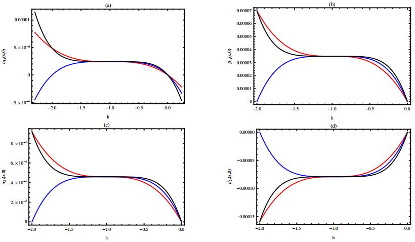
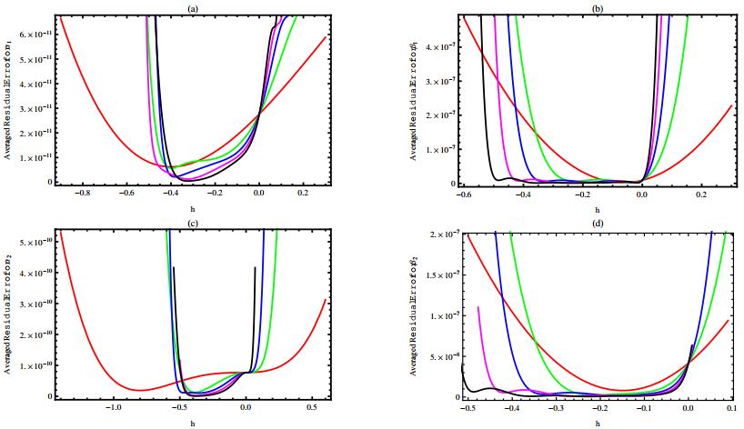
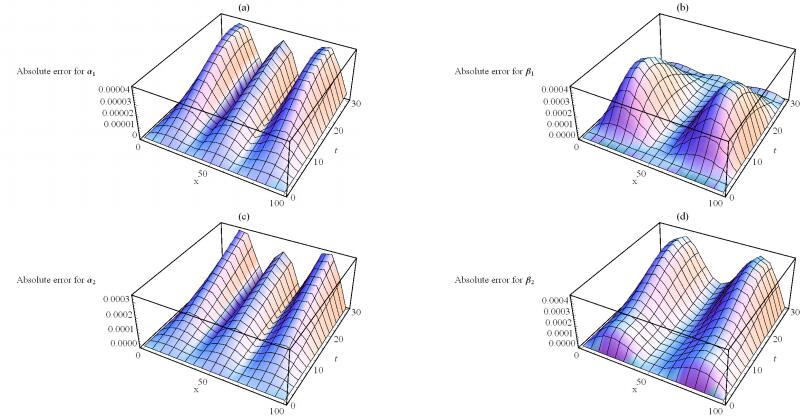
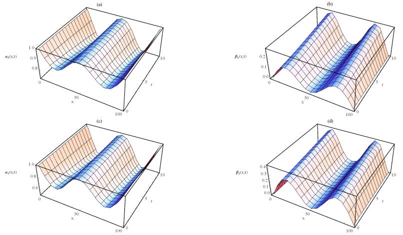
We established an effective algorithm for the homotopy analysis method (HAM) to solve a cubic isothermal auto-catalytic chemical system (CIACS). Our solution comes in a rapidly convergent series where the intervals of convergence given by h-curves and to find the optimal values of h, we used the averaged residual errors. The HAM solutions are compared with the solutions obtained by Mathematica in-built numerical solver. We also show the behavior of the HAM solution.
Citation: K. M. Saad, O. S. Iyiola, P. Agarwal. An effective homotopy analysis method to solve the cubic isothermal auto-catalytic chemical system[J]. AIMS Mathematics, 2018, 3(1): 183-194. doi: 10.3934/Math.2018.1.183
We established an effective algorithm for the homotopy analysis method (HAM) to solve a cubic isothermal auto-catalytic chemical system (CIACS). Our solution comes in a rapidly convergent series where the intervals of convergence given by h-curves and to find the optimal values of h, we used the averaged residual errors. The HAM solutions are compared with the solutions obtained by Mathematica in-built numerical solver. We also show the behavior of the HAM solution.

| [1] | S. Abbasbandy and M. Jalili, Determination of optimal convergence-control parameter value in homotopy analysis method, Numer. Algorithms, 64 (2013), 593-605. |
| [2] | S. Abbasbandya, E. Shivaniana and K. Vajravelub, Mathematical properties of h-curve in the frame work of the homotopy analysis method, Commun. Nonlinear Sci., 16 (2011), 4268-4275. |
| [3] | S. M. Abo-Dahab, S. Mohamed and T. A. Nofal, A One Step Optimal Homotopy Analysis Method for propagation of harmonic waves in nonlinear generalized magneto-thermoelasticity with two relaxation times under influence of rotation, Abstr. Appl. Anal., 2013 (2013), 1-14. |
| [4] | A. Sami Bataineh, M. S. M. Noorani and I. Hashim, The homotopy analysis method for Cauchy reaction diffusion problems, Phys. Lett. A, 372 (2008), 613-618. |
| [5] | K. A. Gepreel and M. S. Mohamed, An optimal homotopy analysis method nonlinear fractional differential equation, Journal of Advanced Research in Dynamical and Control Systems, 6 (2014), 1-10. |
| [6] | M. Ghanbari, S. Abbasbandy and T. Allahviranloo, A new approach to determine the convergencecontrol parameter in the application of the homotopy analysis method to systems of linear equations, Appl. Comput. Math., 12 (2013), 355-364. |
| [7] | J. H. Merkin, D. J. Needham and S. K. Scott, Coupled reaction-diffusion waves in an isothermal autocatalytic chemical system, IMA J. Appl. Math., 50 (1993), 43-76. |
| [8] | O. S. Iyiola, A numerical study of ito equation and Sawada-Kotera equation both of time-fractional type, Adv. Math., 2 (2013), 71-79. |
| [9] | O. S. Iyiola, A fractional diffusion equation model for cancer tumor, American Institute of Physics Advances, 4 (2014), 107121. |
| [10] | O. S. Iyiola, Exact and Approximate Solutions of Fractional Diffusion Equations with Fractional Reaction Terms, Progress in Fractional Di erentiation and Applications, 2 (2016), 21-30. |
| [11] | O. S. Iyiola and G. O. Ojo, On the analytical solution of Fornberg-Whitham equation with the new fractional derivative, Pramana, 85 (2015), 567-575. |
| [12] | O.S. Iyiola, O. Tasbozan, A. Kurt, et al. On the analytical solutions of the system of conformable time-fractional Robertson equations with 1-D diffusion, Chaos, Solitons and Fractals, 94 (2017), 1-7. |
| [13] | S. J. Liao, The proposed homotopy analysis technique for the solution of nonlinear problems, PhD thesis, Shanghai Jiao Tong University, 1992. |
| [14] | S. J. Liao, Beyond perturbation: introduction to the homotopy analysis method, Boca Raton: Chapman and Hall/CRC Press, 2003. |
| [15] | S. J. Liao, An optimal homotopy analysis approach for strongly nonlinear differential equations, Commun. Nonlinear Sci., 15 (2010), 2003-2016. |
| [16] | M. Russo and R. V. Gorder, Control of error in the homotopy analysis of nonlinear Klein-Gordon initial value problems, Appl. Math. Comput., 219 (2013), 6494-6509. |
| [17] | K. M. Saad, An approximate analytical solutions of coupled nonlinear fractional diffusion equations, Journal of Fractional Calculus and Applications, 5 (2014), 58-72. |
| [18] | K. M. Saad, E. H. AL-Shareef, S. Mohamed, et al. Optimal q-homotopy analysis method for timespace fractional gas dynamics equation, Eur. Phys. J. Plus, 132 (2017), 23. |
| [19] | K. M. Saad and A. A. AL-Shomrani, An application of homotopy analysis transform method for riccati differential equation of fractional order, Journal of Fractional Calculus and Applications, 7 (2016), 61-72. |
| [20] | M. Shaban, E. Shivanian and S. Abbasbandy, Analyzing magneto-hydrodynamic squeezing flow between two parallel disks with suction or injection by a new hybrid method based on the Tau method and the homotopy analysis method, Eur. Phys. J. Plus, 128 (2013), 133. |
| [21] | E. Shivanian and S. Abbasbandy, Predictor homotopy analysis method: Two points second order boundary value problems, Nonlinear Anal-Real, 15 (2014), 89-99. |
| [22] | E. Shivanian, H. H. Alsulami, M. S Alhuthali, et al. Predictor Homotopy Analysis Method (Pham) for Nano Boundary Layer Flows with Nonlinear Navier Boundary Condition: Existence of Four Solutions, Filomat, 28 (2014), 1687-1697. |
| [23] | L. A. Soltania, E. Shivanianb and R. Ezzatia, Convection-radiation heat transfer in solar heat exchangers filled with a porous medium: Exact and shooting homotopy analysis solution, Appl. Therm. Eng., 103 (2016), 537-542. |
| [24] | H. Vosoughi, E. Shivanian and S. Abbasbandy, Unique and multiple PHAM series solutions of a class of nonlinear reactive transport model, Numer. Algorithms, 61 (2012), 515-524. |
| [25] | H. Vosughi, E. Shivanian and S. Abbasbandy, A new analytical technique to solve Volterra's integral equations, Math. methods appl. sci., 34 (2011), 1243-1253. |
| [26] | M. Yamashita, K. Yabushita and K. Tsuboi, An analytic solution of projectile motion with the quadratic resistance law using the homotopy analysis method, J. Phys. A, 40 (2007), 8403-8416. |
| [27] | X. Zhang, P. Agarwal, Z. Liu, et al. Existence and uniqueness of solutions for stochastic differential equations of fractional-order q > 1 with finite delays, Adv. Di er. Equ-NY, 123 (2017), 1-18. |
| [28] | M. Ruzhansky, Y. J. Cho, P. Agarwal, et al. Advances in Real and Complex Analysis with Applications, Springer Singapore, 2017. |
| [29] | S. Salahshour, A. Ahmadian, N. Senu, et al. On analytical solutions of the fractional differential equation with uncertainty: application to the Basset problem, Entropy, 17 (2015), 885-902. |
Figures(4) / Tables(4)

K. M. Saad, O. S. Iyiola, P. Agarwal. An effective homotopy analysis method to solve the cubic isothermal auto-catalytic chemical system[J]. AIMS Mathematics, 2018, 3(1): 183-194. doi: 10.3934/Math.2018.1.183


 DownLoad: