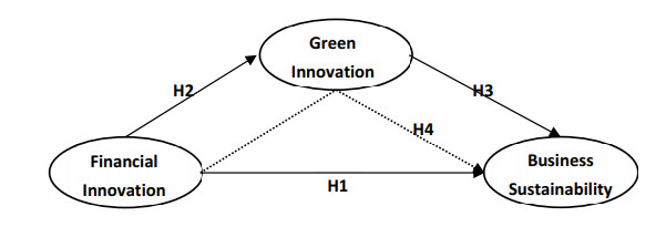
Recent studies have shown that the lack of environmental regulations in public administrations, the inability of employees to innovate knowledge and skills, the high price of green technologies, and the lack of environmental awareness in organizations are the biggest threats to the environmental and sustainable development. In this context, manufacturing companies in emerging markets should not only focus on achieving a higher level of business sustainability in economic and financial terms, but also pay attention to financial and green innovation, because they are important ways to achieve a green transformation of businesses, to improve sustainability, and to reduce carbon dioxide emissions. This study provides data on the adoption and repercussions of these activities on the sustainability of manufacturing companies in Mexico. The proposed research model was validated by applying partial least squares structural equation modeling (PLS-SEM) on a sample of 338 companies. The results of the study showed that the business sustainability of manufacturing companies significantly improved through the application of financial and green innovation. In addition, the results of the study showed that green innovation plays the role of a mediating variable in the relationship between financial innovation and corporate sustainable development.
Citation: Gonzalo Maldonado-Guzmán. Green innovation mediates between financial innovation and business sustainability? Proof in the mexican manufacturing industry[J]. Green Finance, 2024, 6(3): 563-584. doi: 10.3934/GF.2024021
Recent studies have shown that the lack of environmental regulations in public administrations, the inability of employees to innovate knowledge and skills, the high price of green technologies, and the lack of environmental awareness in organizations are the biggest threats to the environmental and sustainable development. In this context, manufacturing companies in emerging markets should not only focus on achieving a higher level of business sustainability in economic and financial terms, but also pay attention to financial and green innovation, because they are important ways to achieve a green transformation of businesses, to improve sustainability, and to reduce carbon dioxide emissions. This study provides data on the adoption and repercussions of these activities on the sustainability of manufacturing companies in Mexico. The proposed research model was validated by applying partial least squares structural equation modeling (PLS-SEM) on a sample of 338 companies. The results of the study showed that the business sustainability of manufacturing companies significantly improved through the application of financial and green innovation. In addition, the results of the study showed that green innovation plays the role of a mediating variable in the relationship between financial innovation and corporate sustainable development.

| [1] |
Abbasi K, Hussain K, Haddad A, et al. (2021) The role of financial development and technological innovation towards sustainable development in Pakistan: Fresh insights from consumption and territory-based emissions. Technol Forecast Soc Chang 176: 1–13. https://doi.org/10.1016/j.techfore.2021.121444 doi: 10.1016/j.techfore.2021.121444

|
| [2] |
Acheampong A, Amponsah M, Boateng E (2020) Does financial development mitigate carbon emissions? Evidence from heterogeneous financial economies. Energ Econ 88: 1–11. https://doi.org/10.1016/j.eneco.2020.104768 doi: 10.1016/j.eneco.2020.104768
|
| [3] |
Ahmed W, Ashraf M, Khan S, et al. (2020) Analyzing the impact of environmental collaboration among supply chain stakeholders on a firm's sustainable performance. Opera Manage Res 13: 4–21. https://doi.org/10.1007/s12063-020-00152-1 doi: 10.1007/s12063-020-00152-1
|
| [4] |
Akram R, Majeed T, Fareed Z, et al. (2020) Asymmetric effects of energy efficiency and renewable energy on carbon emission of BRICS economies: Evidence from nonlinear panel autoregressive distributed lag model. Environ Sci Pollut R 27: 18254–18268. https://doi.org/10.1007/s11356-020-08353-8 doi: 10.1007/s11356-020-08353-8
|
| [5] |
Al-Batayneh A, Khaddam A, Irtaimeh H, et al. (2021) Drivers of performance indicators for success of green SCM strategy and sustainable performance: The mediator role innovation strategy. Int J Serv Sci Manage Eng Technol 12: 14–28. https://doi.org/10.4018/IJSSMET.2021090102 doi: 10.4018/IJSSMET.2021090102
|
| [6] |
Albort-Morant G, Leal-Millán A, Cepeda-Carrión G (2016) The antecedents of green innovation performance: A model learning and capabilities. J Bus Res 69: 4912–4917. https://doi.org/10.1016/j.jbusres.2016.04.052 doi: 10.1016/j.jbusres.2016.04.052
|
| [7] |
Ali W, Jun W, Hussain H, et al. (2021) Does green intellectual capital matter for green innovation adoption? Evidence from the manufacturing SMEs of Pakistan. J Intellect Cap 22: 868–888. https://doi.org/10.1108/JIC-06-2020-0204 doi: 10.1108/JIC-06-2020-0204
|
| [8] |
Andersen J (2021) A relational natural-resource-based view on product innovation: The influence of green product innovation and green suppliers on differentiation advantages in small manufacturing firms. Technovation 104: 1–11. https://doi.org/10.1016/j.technovation.2021.102254 doi: 10.1016/j.technovation.2021.102254
|
| [9] |
Andersson LM, Bateman TS (1997) Cynicism in the workplace: Some causes and effects. J Organ Behav 18: 449–469. https://doi.org/10.1002/(SICI)1099-1379(199709)18:5<449::AID-JOB808>3.0.CO;2-O doi: 10.1002/(SICI)1099-1379(199709)18:5<449::AID-JOB808>3.0.CO;2-O
|
| [10] |
Anees S, Zaidi H, Hussain M, et al. (2021) Resources, environment and sustainability dynamic linkages between financial inclusion and carbon emission: Evidence from selected OECD countries. Resour Environ Sustain 4: 1–12. https://doi.org/10.1016/j.resenv.2021.100022 doi: 10.1016/j.resenv.2021.100022
|
| [11] |
Anwar A, Siddique M, Dogan E, et al. (2021) The moderating role of renewable and non-renewable energy in environment-income nexus for ASEAN countries: Evidence from method of moments quantile regression. Renew Energ 164: 956–967. https://doi.org/10.1016/j.renene.2020.09.128 doi: 10.1016/j.renene.2020.09.128
|
| [12] |
Arnold M, Schuette D, Wagner A (2021) Neglected risk in financial innovation: Evidence from structured product counterparty exposure. Eur Financ Manag 27: 287–325. https://doi.org/10.1111/eufm.12281 doi: 10.1111/eufm.12281
|
| [13] |
Astuti D, Datrini L (2021) Green competitive advantage: Examining the role of environmental consciousness and green intellectual capital. Manage Sci Lett 11: 1141–1152. https://doi.org/10.5267/j.msl.2020.11.025 doi: 10.5267/j.msl.2020.11.025
|
| [14] |
Aulakh PS, Gencturk EF (2000) International principal-agent relationships-control, governance and performance. Ind Market Manag 29: 521–538. https://doi.org/10.1016/S0019-8501(00)00126-7 doi: 10.1016/S0019-8501(00)00126-7
|
| [15] |
Barney J (1991) Firm resources and sustained competitive advantage. J Manage 17: 99–120. https://doi.org/10.1177/014920639101700108 doi: 10.1177/014920639101700108
|
| [16] | Biswas S (2020) Al-Bank of the Future: Can Banks Meet the AI Challenge? New York: McKinsey and Co. |
| [17] | Bond C (2020) 6 predictions for banking in 2021. US News, 23 December. Available from: https://money.usnews.com/banking/articles/predictions-for-banking. |
| [18] |
Cai W, Li G (2018) The drivers of eco-innovation and its impact on performance: Evidence from China. J Clean Prod 176: 110–118. https://doi.org/10.1016/j.jclepro.2017.12.109 doi: 10.1016/j.jclepro.2017.12.109
|
| [19] | Castelli B (2019) Machine Learning: What Every Risk and Compliance Professional Needs to Know. PWC. Available from: https://www.pwc.com/us/en/services/consulting/cybersecurity-privacy-forensics/library/machine-learning-risk-compliance.html. |
| [20] |
Cepeda-Carrion G, Cegarra J, Cillo V (2019) Tips to use partial least squares structural equation modelling (PLS-SEM) in knowledge management. J Knowl Manag 23: 67–89. https://doi.org/10.1108/JKM-05-2018-0322 doi: 10.1108/JKM-05-2018-0322
|
| [21] |
Chang X, Chen Y, Wang S, et al. (2019) Credit default swaps and corporate innovation. J Financ Econ 134: 474–500. https://doi.org/10.1016/j.jfineco.2017.12.012 doi: 10.1016/j.jfineco.2017.12.012
|
| [22] |
Chen M, Wang H, Wang M (2018a) Knowledge sharing, social capital, and financial performance: The perspective of innovation strategy in technological clusters. Knowl Man Res Pract 16: 89–104. https://doi.org/10.1080/14778238.2017.1415119 doi: 10.1080/14778238.2017.1415119
|
| [23] |
Chen Z, Huang S, Liu C, et al. (2018b) Fit between organizational culture and innovation strategy: Implications for innovation performance. Sustainability 10: 1–18. https://doi.org/10.3390/su10103378 doi: 10.3390/su10103378
|
| [24] |
Deluca H, Wagner M, Block J (2018) Sustainability and environmental behavior in family firms: A longitudinal analysis of environment related activities, innovation, and performance. Bus Strat Environ 27: 152–172. https://doi.org/10.1002/bse.1998 doi: 10.1002/bse.1998
|
| [25] |
Farkavcova V, Rieckhof R, Guenther E (2018) Expanding knowledge environmental impacts of transport processes for more sustainable supply chain decisions: A case study using life cycle assessment. Transport Res D-TR E 61: 68–83. https://doi.org/10.1016/j.trd.2017.04.025 doi: 10.1016/j.trd.2017.04.025
|
| [26] |
Fatoki O (2021) Environmental orientation and green competitive advantage of hospitality firms in South Africa: mediating effect of green innovation. J Open Innov Technol Market Complex 7: 1–14. https://doi.org/10.3390/joitmc7040223 doi: 10.3390/joitmc7040223
|
| [27] |
Fernando Y, Chiappetta-Jabbour C, Wah W (2019) Pursuing green growth in technology firms through the connections between environmental innovation and sustainable business performance: Does service capability matter? Resour Conserv Recy 141: 8–20. https://doi.org/10.1016/j.resconrec.2018.09.031 doi: 10.1016/j.resconrec.2018.09.031
|
| [28] |
Gathergood J, Weber J (2017) Financial literacy, present bias, and alternative mortgage products. J Bank Financ 78: 58–83. https://doi.org/10.1016/j.jbankfin.2017.01.022 doi: 10.1016/j.jbankfin.2017.01.022
|
| [29] |
Gennaioli N, Shleifer A, Vishny R (2012) Neglected risks, financial innovation, and financial fragility. J Financ Econ 104: 452–468. https://doi.org/10.1016/j.jfineco.2011.05.005 doi: 10.1016/j.jfineco.2011.05.005
|
| [30] |
González L, Gil L, Cunill O, et al. (2016) The effect of financial innovation on European banks risk. J Bank Res 69: 4781–4786. https://doi.org/10.1016/j.jbusres.2016.04.030 doi: 10.1016/j.jbusres.2016.04.030
|
| [31] |
Gürlek M, Tuna M (2018) Reinforcing competitive advantage through green organizational culture and green innovation. Serv Ind J 38: 467–491. https://doi.org/10.1080/02642069.2017.1402889 doi: 10.1080/02642069.2017.1402889
|
| [32] | Hair J, Hult T, Ringle C, et al. (2019) Manual de Partial Least Squares PLS-SEM. Madrid: OmniaScience. Available from: http://hdl.handle.net/11420/5279. |
| [33] |
Hair J, Sarstedt M (2021) Data, measurement, and causal inferences in machine learning: Opportunities and challenges for marketing. J Market Theory Prac 29: 65–77. https://doi.org/10.1080/10696679.2020.1860683 doi: 10.1080/10696679.2020.1860683
|
| [34] |
Hair J, Howard M, Nitzl C (2020) Assessing measurement model quality in PLS-SEM using confirmatory composite analysis. J Bus Res 109: 101–110. https://doi.org/10.1016/j.jbusres.2019.11.069 doi: 10.1016/j.jbusres.2019.11.069
|
| [35] |
Hair J, Hult G, Ringle C, et al. (2017) Mirror, mirror on the wall: A comparative evaluation of composite-based structural equation modeling methods. J Acad Market Sci 45: 616–632. https://doi.org/10.1007/s11747-017-0517-x doi: 10.1007/s11747-017-0517-x
|
| [36] | Hair JF, Celsi M, Money A, et al. (2016) Essentials of Business Research Methods. 3rd Ed. New York, NY: Routledge. https://doi.org/10.4324/9781315704562 |
| [37] |
Hart S (1995) A natural-resource-based view of the firm. Acad Manage Rev 20: 986–1014. https://doi.org/10.5465/amr.1995.9512280033 doi: 10.5465/amr.1995.9512280033
|
| [38] |
Henseler J (2018) Partial least squares path modeling: Quo vadis? Qual Quant 52: 1–8. https://doi.org/10.1007/s11135-018-0689-6 doi: 10.1007/s11135-018-0689-6
|
| [39] |
Hu J, Li J, Li X, et al. (2021) Will green finance contribute to a green recovery? Evidence from green financial pilot zone in China. Frontiers Public Health 9: 1–15. https://doi.org/10.3389/fpubh.2021.794195 doi: 10.3389/fpubh.2021.794195
|
| [40] |
Huang J, Li Y (2017) Green innovation and performance: The view of organizational capability and social reciprocity. J Bus Ethics 145: 309–324. https://doi.org/10.1007/s10551-015-2903-y doi: 10.1007/s10551-015-2903-y
|
| [41] |
Huang P, Yao C, Chen S (2019a) Development of the organizational resources towards innovation strategy and innovation value: Empirical study. Revista de Cercetare si Interventie Sociala 64: 108–119. https://doi.org/10.33788/rcis.64.9 doi: 10.33788/rcis.64.9
|
| [42] |
Huang Z, Liao G, Li Z (2019b) Loaning scale and government subsidy for promoting green innovation. Technol Forecast Soc Chang 144: 148–156. https://doi.org/10.1016/j.techfore.2019.04.023 doi: 10.1016/j.techfore.2019.04.023
|
| [43] | Huber N (2020) AI only scratching the surface of potential in finance services. Financ Times. Available from: https://www.ft.com/content/11aab1cc-907b-11ea-bc44-dbf6756c871a. |
| [44] | INEGI (2021) Directorio Estadístico Nacional de Unidades Económicas. Available from: https://www.inegi.org.mx/app/mapa/denue/default.aspx. |
| [45] | Instituto Nacional de Estadística y Geografía[INEGI]. (2023) Banco de Indicadores. Producción Bruta Total. Industrias Manufactureras. Available from: https://www.inegi.org.mx/app/indicadores/?t = 261 & ag = 01#D261. |
| [46] |
Iverson RD, Maguire C (2000) The relationship between job and life satisfaction: Evidence from a remote mining community. Hum Relat 53: 807–839. https://doi.org/10.1177/0018726700536003 doi: 10.1177/0018726700536003
|
| [47] |
Jahanger A, Usman M, Murshed M, et al. (2022) The linkage between natural resources, human capital, globalization, economic growth, financial development, and ecological footprint: The moderating role of technological innovation. Resour Policy 76: 1–12. https://doi.org/10.1016/j.resourpol.2022.102569 doi: 10.1016/j.resourpol.2022.102569
|
| [48] |
Jiang W, Chai H, Shao J, et al. (2018) Green entrepreneurial orientation for enhancing firm performance: A dynamic capability perspective. J Clean Prod 198: 1311–1323. https://doi.org/10.1016/j.jclepro.2018.07.104 doi: 10.1016/j.jclepro.2018.07.104
|
| [49] |
Jin C, Shahzad M, Zafar A, et al. (2022) Socio-economic and environmental drivers of green innovation: Evidence from nonlinear ARDL. Econ Res-Ekonomska Istrazivanja 35: 5336–5356. https://doi.org/10.1080/1331677X.2022.2026241 doi: 10.1080/1331677X.2022.2026241
|
| [50] |
Karami M, Madlener R (2021) Business model innovation for the energy market: Joint value creation for electricity retailers and their customers. Energy Res Soc Sci 73: 1–12. https://doi.org/10.1016/j.erss.2020.101878 doi: 10.1016/j.erss.2020.101878
|
| [51] | Kemp R, Pearson P (2008) MEI project about measuring eco-innovation. J Sci Technology Inf 2: 85–95. |
| [52] |
Kim J, Park K (2016) Financial development and deployment of renewable energy technologies. Energ Econ 59: 238–250. https://doi.org/10.1016/j.eneco.2016.08.012 doi: 10.1016/j.eneco.2016.08.012
|
| [53] |
Laeven L, Levine R, Michalopoulos S (2015) Financial innovation and endogenous growth. J Financ Intermed 24: 1–24. https://doi.org/10.1016/j.jfi.2014.04.001 doi: 10.1016/j.jfi.2014.04.001
|
| [54] |
Le TT (2022) How do corporate social responsibility and green innovation transform corporate green strategy into sustainable firm performance? J Clean Prod 362. https://doi.org/10.1016/j.jclepro.2022.132228 doi: 10.1016/j.jclepro.2022.132228
|
| [55] |
Le T, Le H, Taghizadeh-Hesary F (2020) Does financial inclusion impact CO2 emissions? Evidence from Asia. Financ Res Lett 34: 1–13. https://doi.org/10.1016/j.frl.2020.101451 doi: 10.1016/j.frl.2020.101451
|
| [56] |
Lepistö K, Saunila M, Ukko J (2023) The effects of soft total quality management on the sustainable developments of SMEs. Sustain Dev 31: 2797–2813. https://doi.org/10.1002/sd.2548 doi: 10.1002/sd.2548
|
| [57] |
Li D, Zheng M, Cao C, et al. (2017) The impact of the legitimacy pressure and corporate profitability on green innovation: Evidence from China top 100. J Clean Prod 141: 41–49. https://doi.org/10.1016/j.jclepro.2016.08.123 doi: 10.1016/j.jclepro.2016.08.123
|
| [58] |
Li W, Bhutto M, Waris I, et al. (2023) The nexus between environmental corporate social responsibility, green intellectual capital, and green innovation towards business sustainability: An empirical analysis of Chinese automobile manufacturing firms. Int J Env Res Pub He 20: 1–20. https://doi.org/10.3390/ijerph20031851 doi: 10.3390/ijerph20031851
|
| [59] |
Lin H, Chen L, Yu M, et al. (2021) Too little or too much of good things? The horizontal S-curve hypothesis of green business strategy on firm performance. Technol Forecast Soc 172. https://doi.org/10.1016/j.techfore.2021.121051 doi: 10.1016/j.techfore.2021.121051
|
| [60] |
Liu S, Wang Y (2023) Green innovation effect of pilot zone for green finance reform: Evidence of quasi natural experiment. Technol Forecast Soc 186: 1–10. https://doi.org/10.1016/j.techfore.2022.122079 doi: 10.1016/j.techfore.2022.122079
|
| [61] |
Liu Y, Lei J, Zhang Y (2021) A study on the sustainable relationship among the green finance, environmental regulation, and green-total-factor productivity in China. Sustainability 13: 1–27. https://doi.org/10.3390/su132111926 doi: 10.3390/su132111926
|
| [62] |
Lopez-Torres GC (2023) The impact of SMEs' sustainability on competitiveness. Meas Bus Excell 27: 107–120. https://doi.org/10.1108/MBE-12-2021-0144 doi: 10.1108/MBE-12-2021-0144
|
| [63] | Maingi M, Wanjiru G, Samuel K, et al. (2013) Financial innovation as a competitive strategy: The Kenyan financial sector. J Modern Accounting Auditing 9: 997–1004. http://repository.rongovarsity.ac.ke/handle/123456789/747 |
| [64] | Maldonado-Guzmán G, Pinzón SY, Alvarado A (2020) Responsabilidad Social Empresarial, Ecoinnovación y Rendimiento Sustentable en la Industria Automotriz de México. Revista Venezolana de Gerencia, 25: 188–205. Available from: https://www.redalyc.org/articulo.oa?id=29062641014%0APDF. |
| [65] | Mbogoh G (2013) The effect of financial innovation on financial performance of insurance companies in Kenya. Doctoral dissertation, University of Nairobi. |
| [66] | McKinsey (2020) How Covid-19 has Pushed Companies over the Technology Tipping Point: An Transformed Business Forever. McKinsey and Co. Available from: https://www.mckinsey.com/business-functions/strategy-an-corporate-finance/our-insights/how-covid-19-has-pushed-companies-over-the-technology-tipping-point-and-transformed-business-forever. |
| [67] |
Mohd S, Mohd S, Sharif A, et al. (2022) Importance of green innovation for business sustainability: Identifying the key role of green intellectual capital and green SCM. Bus Strateg Environ 32: 1542–1558. https://doi.org/10.1002/bse.3204 doi: 10.1002/bse.3204
|
| [68] |
Mossholder KW, Bennett N, Kemery ER, et al. (1998) Relationships between bases of power and work reactions: The mediational role of procedural justice. J Manage 24: 533–552. https://doi.org/10.1016/S0149-2063(99)80072-5 doi: 10.1016/S0149-2063(99)80072-5
|
| [69] |
Naeem M, Conlon T, Cotter J (2022) Green bonds and other assets. Evidence from extreme risk transmission. J Environ Manage 305: 1–12. https://doi.org/10.1016/j.jenvman.2021.114358 doi: 10.1016/j.jenvman.2021.114358
|
| [70] |
Najmi A, Kanapathy K, Aziz A (2019) Prioritizing factor influencing consumers' reversing intention of e-waste using analytic hierarchy process. Int J Electron Customer Relationship Manage 12: 58–74. https://doi.org/10.1504/IJECRM.2019.098981 doi: 10.1504/IJECRM.2019.098981
|
| [71] |
Nejad G (2022) Research on financial innovations: An interdisciplinary review. Int J Bank Mark 40: 578–612. https://doi.org/10.1108/IJBM-07-2021-0305 doi: 10.1108/IJBM-07-2021-0305
|
| [72] |
Nejad G (2016) Research on financial services innovations: A quantitative review and future research directions. Int J Bank Mark 34: 1042–1067. https://doi.org/10.1108/IJBM-08-2015-0129 doi: 10.1108/IJBM-08-2015-0129
|
| [73] | Noailly J, Smeets R (2016) Financing energy innovation: The role of financing constraints for direct technical change from fossil-fuel to renewable innovation. EIB Working Papers No. 216/06. Luxembourg: European Investment Bank (EIB) Available from: http://hdl.handle.net/10419/148571. |
| [74] | Ortiz-Palafox KH (2019) Sustentabilidad como estrategia competitiva en la gerencia de pequeñas y medianas empresas en México. Revista Venezolana de Gerencia 24: https://www.redalyc.org/jatsRepo/290/29062051001/ |
| [75] |
Pham L (2019) Does financial development matter for innovation in renewable energy? Appl Econ Lett 26: 1756–1761. https://doi.org/10.1080/13504851.2019.1593934 doi: 10.1080/13504851.2019.1593934
|
| [76] |
Podsakoff PM, MacKenzie SB, Podsakoff NP (2012) Sources of method bias in social science research and recommendations on how to control it. Annu Rev Psychol 63: 539–569. https://doi.org/10.1146/annurev-psych-120710-100452 doi: 10.1146/annurev-psych-120710-100452
|
| [77] |
Podsakoff PM, MacKenzie SB, Jeong-Yeong L, et al. (2003) Common method biases in behavioral research: A critical review of the literature and recommended remedies. J Appl Psychol 88: 879–903. https://doi.org/10.1037/0021-9010.88.5.879 doi: 10.1037/0021-9010.88.5.879
|
| [78] |
Qiu L, Jie X, Wang Y, et al. (2020) Green product innovation, green dynamic capability, and competitive advantage: Evidence from Chinese manufacturing enterprises. Corp Soc Resp Env Ma 27: 146–165. https://doi.org/10.1002/csr.1780 doi: 10.1002/csr.1780
|
| [79] |
Qu C, Shao J, Shi Z (2020) Does financial agglomeration promote the increase of energy efficiency in China? Energ Policy 146: 1–12. https://doi.org/10.1016/j.enpol.2020.111810 doi: 10.1016/j.enpol.2020.111810
|
| [80] |
Rehman S, Kraus S, Shah S, et al. (2021) Analyzing the relationship between green innovation and environmental performance in large manufacturing firms. Technol Forecast Soc 163: 1–13. https://doi.org/10.1016/j.techfore.2020.120481 doi: 10.1016/j.techfore.2020.120481
|
| [81] |
Ringle C, Sarstedt M, Mitchell R, et al. (2020) Partial least squares structural equation modeling in HRM research. Int J Human Resour Manage 31: 1617–1643. https://doi.org/10.1080/09585192.2017.1416655 doi: 10.1080/09585192.2017.1416655
|
| [82] | Ringle C, Wende S, Becker J (2022) SmartPLS 4 (computer software). Available from: http://www.smartpls.com. |
| [83] |
Rodríguez-Espíndola O, Cuevas-Romo A, Chowdhury S, et al. (2022) The role of circular economy principles and sustainable-oriented innovation to enhance social, economic and environmental performance: Evidence from Mexican SMEs. Int J Prod Econ 248. https://doi.org/10.1016/j.ijpe.2022.108495 doi: 10.1016/j.ijpe.2022.108495
|
| [84] |
Rodríguez-González RM, Maldonado-Guzman G, Madrid-Guijarro A (2022) The effect of green strategies and eco-innovation on Mexican automotive industry sustainable and financial performance: Sustainable supply chains as a mediating variable. Corp Soc Resp Env Ma 29: 779–794. https://doi.org/10.1002/csr.2233 doi: 10.1002/csr.2233
|
| [85] |
Ronaldo R, Suryanto T (2022) Green finance and sustainability development goals in Indonesian Fund Village. Resour Policy 78: 1–12. https://doi.org/10.1016/j.resourpol.2022.102839 doi: 10.1016/j.resourpol.2022.102839
|
| [86] | Sachs J, Woo W, Yoshino N, et al. (2019) Importance of green finance for achieving sustainable development goals and energy security, In: Sachs J. (Ed.), Handbook of Green Finance: Energy Security and Sustainable Development, Japan: CiNii, 3–12. https://doi.org/10.1007/978-981-13-0227-5_13 |
| [87] | Sardon M (2020) Millennials prefer apps to humans for financial advice. Wall Street J, 16 March. Available from: https://www.wsj.com/articles/millennials-prefer-apps-to-humans-for-financial-advice-11584377127. |
| [88] |
Sarstedt M, Hair JF, Ringle CM, et al. (2016) Estimation issues with PLS and CBSEM: Where the bies lies. J Bus Res 69: 3998–4010. https://doi.org/10.1016/j.jbusres.2016.06.007 doi: 10.1016/j.jbusres.2016.06.007
|
| [89] |
Sarstedt M, Hair J, Cheah J, et al. (2019) How to specify, estimate, and validate higher-order constructs in PLS-SEM. Australas Mark J (AMJ) 27: 197–211. https://doi.org/10.1016/j.ausmj.2019.05.003. doi: 10.1016/j.ausmj.2019.05.003
|
| [90] |
Saunila M, Ukko J, Rantala T (2018) Sustainability as a driver of green innovation investment and exploitation. J Clean Prod 179: 631–641. https://doi.org/10.1016/j.jclepro.2017.11.211 doi: 10.1016/j.jclepro.2017.11.211
|
| [91] |
Scott S, Van Reenen J, Zachariadis M (2017) The long-term effect of digital innovation on bank performance: An empirical study of swift adoption in financial services. Res Policy 46: 984–1004. https://doi.org/10.1016/j.respol.2017.03.010 doi: 10.1016/j.respol.2017.03.010
|
| [92] |
Scur G, de Mello A, Schreiner L, et al. (2019) Eco-design requirements in heavyweight vehicle development – a case study of the impact of the Euro 5 emissions standard on the Brazilian industry. Innov Manage Rev 16: 404–442. https://doi.org/10.1108/INMR-08-2018-0063 doi: 10.1108/INMR-08-2018-0063
|
| [93] |
Shahzad M, Qu Y, Rehman S, et al. (2022) Impact of stakeholder's pressure on green management practices of manufacturing organizations under the mediation of organizational motives. J Environ Plann Manage 66: 2171–2194. https://doi.org/10.1080/09640568.2022.2062567 doi: 10.1080/09640568.2022.2062567
|
| [94] |
Shahzad M, Qu Y, Zafar A, et al. (2021) Does the interaction between the knowledge management process and sustainable development practices boost corporate green innovation? Bus Strateg Environ 30: 1–17. https://doi.org/10.1002/bse.2865 doi: 10.1002/bse.2865
|
| [95] |
Sonmez C, Adiguzel Z (2022) An examination of the effects of financial and process innovation on the sustainability of businesses under the influence of entrepreneurial leadership: A research in energy companies. Am J Bus 37: 196–213. https://doi.org/10.1108/AJB-03-2022-0046 doi: 10.1108/AJB-03-2022-0046
|
| [96] |
Sonmez C, Adiguzel Z (2023) Effects of innovation finance, strategy, organization, and performance: A case study of company. Int J Innov Sci 15: 42–58. https://doi.org/10.1108/IJIS-08-2021-0146 doi: 10.1108/IJIS-08-2021-0146
|
| [97] | Statista (2023) La Industria Manufacturera En México. Datos Estadísticos. Statista Research Department. Available from: https://es.statista.com/temas/7853/la-industria-manufacturera-en-mexico/#topicOvervi. |
| [98] | Streeter B (2020) Four ways banks must change before millennials and Gen Z will love you. The Financial Brand. Available from: https://thefinancialbrand.com/103616/banks-millennials-gen-z-personalization-loyalty-fintech-gamification/. |
| [99] |
Stucki T (2019) Which firms benefit from investments in green energy technologies? The effect of energy costs. Res Policy 48: 546–555. https://doi.org/10.1016/j.respol.2018.09.010 doi: 10.1016/j.respol.2018.09.010
|
| [100] |
Sun Y, Guan W, Razzaq A, et al. (2022b) Transition towards ecological sustainability through fiscal decentralization, renewable energy, and green investment in OECD countries. Renew Energ 190: 385–395. https://doi.org/10.1016/j.renene.2022.03.099 doi: 10.1016/j.renene.2022.03.099
|
| [101] |
Sun Y, Razzaq A, Sun H, et al. (2022a) The asymmetric influence of renewable energy and green innovation on carbon neutrality in China: Analysis from non-linear ARDL model. Renew Energ 193: 334–343. https://doi.org/10.1016/j.renene.2022.04.159 doi: 10.1016/j.renene.2022.04.159
|
| [102] |
Tariq M, Khan I, Rizwan M, et al. (2019) Nexus between financial development, tourism, renewable energy, and greenhouse gas emission in high-income countries: A continent-wise analysis. Energ Econ 83: 293–310. https://doi.org/10.1016/j.eneco.2019.07.018 doi: 10.1016/j.eneco.2019.07.018
|
| [103] |
Tufano P (2003) Financial innovation. Handbook Econ Financ 1: 307–335. https://doi.org/10.1016/S1574-0102(03)01010-0 doi: 10.1016/S1574-0102(03)01010-0
|
| [104] |
Ullah H, Wang Z, Abbas M, et al. (2021b) Association of financial distress and predicted bankruptcy: The case of Pakistani Banking Sector. J Asian Financ Econ Bus 8: 573–585. https://doi.org/10.13106/jafeb.2021.vol8.no1.573 doi: 10.13106/jafeb.2021.vol8.no1.573
|
| [105] |
Ullah H, Wang Z, Bashir S, et al. (2021a) Nexus between IT capability and green intellectual capital on sustainable businesses: Evidence from emerging economies. Environ Sci Pollut Res 28: 27825–27843. https://doi.org/10.1007/s11356-020-12245-2 doi: 10.1007/s11356-020-12245-2
|
| [106] |
Ullah H, Wang Z, Mohsin M, et al. (2022) Multidimensional perspective of green financial innovation between green intellectual capital on sustainable business: The case of Pakistan. Environ Sci Pollut Res 29: 5552–5568. https://doi.org/10.1007/s11356-021-15919-7 doi: 10.1007/s11356-021-15919-7
|
| [107] |
Wang K, Umar M, Akram R, et al. (2021) Is technological innovation making world greener? Evidence from changing growth story of China. Technol Forecast Soc 165: 1–13. https://doi.org/10.1016/j.techfore.2020.120516 doi: 10.1016/j.techfore.2020.120516
|
| [108] |
Wang R, Mirza N, Vasbieva D, et al. (2020a) The nexus of carbon emissions, financial development, renewable energy consumption, and technological innovation: What should be the priorities considering COP21 agreements? J Environ Manage 271: 1–13. https://doi.org/10.1016/j.jenvman.2020.111027 doi: 10.1016/j.jenvman.2020.111027
|
| [109] |
Wang X, Zhao Y, Hou L (2020b) How does green innovation affect supplier-customer relationships? A study on customer and relationship contingencies. Ind Mark Manage 90: 170–180. https://doi.org/10.1016/j.indmarman.2020.07.008 doi: 10.1016/j.indmarman.2020.07.008
|
| [110] |
Wang Y, Yang Y (2021) Analyzing the green innovation practices based on sustainability performance indicators: a Chinese manufacturing industry case. Environ Sci Pollut Res 28: 1181–1203. https://doi.org/10.1007/s11356-020-10531-7 doi: 10.1007/s11356-020-10531-7
|
| [111] |
Xie X, Huo J, Zou H (2019) Green process innovation, green product innovation, and corporate financial performance: A content analysis method. J Bus Res 101: 697–707. https://doi.org/10.1016/j.jbusres.2019.01.010 doi: 10.1016/j.jbusres.2019.01.010
|
| [112] |
Yousaf Z (2021) Go for green: Green innovation through green dynamic capabilities: Accessing the mediate role of green practices and green value. Environ Sci Pollut Res 28: 54863–54875. https://doi.org/10.1007/s11356-021-14343-1 doi: 10.1007/s11356-021-14343-1
|
| [113] |
Yu C, Wu X, Zhang D, et al. (2021) Demand for green finance: Resolving financing constraints on green innovation in China. Energ Policy 153: 1–11. https://doi.org/10.1016/j.enpol.2021.112255 doi: 10.1016/j.enpol.2021.112255
|
| [114] |
Yuan G, Ye Q, Sun Y (2021) Financial innovation, information screening and industries green innovation: Industry-level evidence from the OECD. Technol Forecast Soc 171: 1–12. https://doi.org/10.1016/j.techfore.2021.120998 doi: 10.1016/j.techfore.2021.120998
|
| [115] |
Yue S, Lu R, Shen Y, et al. (2019) How does financial development affect energy consumption? Evidence from 21 transitional countries. Energ Policy 130: 253–262. https://doi.org/10.1016/j.enpol.2019.03.029 doi: 10.1016/j.enpol.2019.03.029
|
| [116] |
Yusliza M, Yong J, Tanveer M, et al. (2020) A structural model of the impact of green intellectual capital on sustainable performance. J Clean Prod 249: 1–14. https://doi.org/10.1016/j.jclepro.2019.119334 doi: 10.1016/j.jclepro.2019.119334
|
| [117] |
Zhang D, Rong Z, Ji Q (2019) Green innovation and firm performance: Evidence from listed companies in China. Resour Conserv Recy 144: 48–55. https://doi.org/10.1016/j.resconrec.2019.01.023 doi: 10.1016/j.resconrec.2019.01.023
|
| [118] |
Zhang X, Yang H, Kumar N, et al. (2023) Assessing Chinese textile and apparel industry business sustainability: The role of organizational green culture, green dynamic capabilities, and green innovation in relation to environmental orientation and business sustainability. Sustainability 15: 1–21. https://doi.org/10.3390/su15118588 doi: 10.3390/su15118588
|
| [119] |
Zhao J, Shahzad M, Dong X, et al. (2021) How does financial risk affect global CO2 emissions? The role of technological innovation. Technol Forecast Soc 168: 14–22. https://doi.org/10.1016/j.techfore.2021.120751 doi: 10.1016/j.techfore.2021.120751
|
| [120] |
Zhou M, Li X (2022) Influence of green finance and renewable energy resources over the sustainable development goals of clean energy. Resourc Policy 78: 13–22. https://doi.org/10.1016/j.resourpol.2022.102816 doi: 10.1016/j.resourpol.2022.102816
|
Figures(1) / Tables(3)

Gonzalo Maldonado-Guzmán. Green innovation mediates between financial innovation and business sustainability? Proof in the mexican manufacturing industry[J]. Green Finance, 2024, 6(3): 563-584. doi: 10.3934/GF.2024021


 DownLoad: