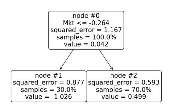
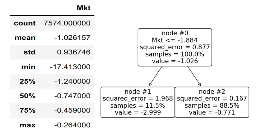
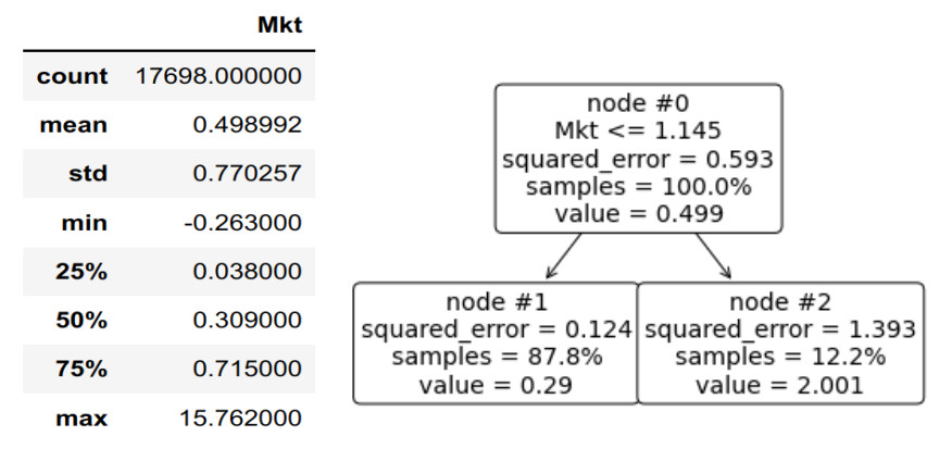
Regression trees (RT) involve sorting samples based on a particular feature and identifying the splitting point that yields the highest drop in variance from a parent node to its children. The optimal factor for reducing mean squared error (MSE) is the target variable itself. Consequently, employing the target variable as the basis for splitting sets an upper limit on the reduction of MSE and, equivalently, a lower limit on the residual MSE. Building upon this observation, we define lepto-regression as the process of constructing an RT of a target feature on itself. Lepto-variance pertains to the portion of variance that cannot be mitigated by any regression tree, providing a measure of inherent variance at a specific tree depth. This concept is valuable as it offers insights into the intrinsic structure of the dataset by establishing an upper boundary on the "resolving power" of RTs for a sample. The maximal variance that can be accounted for by RTs with depths up to k is termed the sample k-bit macro-variance. At each depth, the overall variance within a dataset is thus broken into lepto- and macro-variance. We perform 1- and 2-bit lepto-variance analysis for the entire US stock universe for a large historical period since 1926. We find that the optimal 1-bit split is a 30–70 balance. The two children subsets are centered roughly at −1% and 0.5%. The 1-bit macro-variance is almost 42% of the total US stock variability. The other 58% is structure beyond the resolving power of a 1-bit RT. The 2-bit lepto-variance equals 26.3% of the total, with 42% and 47% of the 1-bit lepto-variance of the left and right subtree, respectively.
Citation: Vassilis Polimenis. The historical lepto-variance of the US stock returns[J]. Data Science in Finance and Economics, 2024, 4(2): 270-284. doi: 10.3934/DSFE.2024011
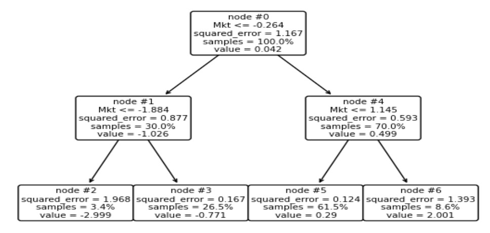
Regression trees (RT) involve sorting samples based on a particular feature and identifying the splitting point that yields the highest drop in variance from a parent node to its children. The optimal factor for reducing mean squared error (MSE) is the target variable itself. Consequently, employing the target variable as the basis for splitting sets an upper limit on the reduction of MSE and, equivalently, a lower limit on the residual MSE. Building upon this observation, we define lepto-regression as the process of constructing an RT of a target feature on itself. Lepto-variance pertains to the portion of variance that cannot be mitigated by any regression tree, providing a measure of inherent variance at a specific tree depth. This concept is valuable as it offers insights into the intrinsic structure of the dataset by establishing an upper boundary on the "resolving power" of RTs for a sample. The maximal variance that can be accounted for by RTs with depths up to k is termed the sample k-bit macro-variance. At each depth, the overall variance within a dataset is thus broken into lepto- and macro-variance. We perform 1- and 2-bit lepto-variance analysis for the entire US stock universe for a large historical period since 1926. We find that the optimal 1-bit split is a 30–70 balance. The two children subsets are centered roughly at −1% and 0.5%. The 1-bit macro-variance is almost 42% of the total US stock variability. The other 58% is structure beyond the resolving power of a 1-bit RT. The 2-bit lepto-variance equals 26.3% of the total, with 42% and 47% of the 1-bit lepto-variance of the left and right subtree, respectively.

| [1] |
Aloise D, Deshpande A, Hansen P, et al. (2009) NP-hardness of Euclidean sum-of-squares clustering. Mach Learn 75: 245–248. https://doi.org/10.1007/s10994-009-5103-0 doi: 10.1007/s10994-009-5103-0

|
| [2] |
Ang A, Hodrick RJ, Xing Y, et al. (2006) The cross-section of volatility and expected returns. J Financ 61: 259–299. https://doi.org/10.1111/j.1540-6261.2006.00836.x doi: 10.1111/j.1540-6261.2006.00836.x
|
| [3] | Breiman L, Friedman J, Olshen R, et al. (1984) Classification and Regression Trees. Wadsworth, Belmont, CA |
| [4] |
Campbell JY, Lettau M, Malkiel BG, et al. (2001) Have Individual Stocks Become More Volatile? An Empirical Exploration of Idiosyncratic Risk. J Financ 56: 1–43. https://doi.org/10.1111/0022-1082.00318 doi: 10.1111/0022-1082.00318
|
| [5] |
Demeterfi K, Derman E, Kamal M, et al. (1999) A Guide to Volatility and Variance Swaps. J Deriv 6: 9–32. https://doi.org/10.3905/jod.1999.319129 doi: 10.3905/jod.1999.319129
|
| [6] |
Elith J, Leathwick JR, Hastie T (2008) A working guide to boosted regression trees. J Anim Ecol 77: 802–813. https://doi.org/10.1111/j.1365-2656.2008.01390.x doi: 10.1111/j.1365-2656.2008.01390.x
|
| [7] |
Fama EF, French KR (1993) Common Risk Factors in the Returns on Stocks and Bonds. J Financ Econ 33: 3–56. https://doi.org/10.1016/0304-405X(93)90023-5 doi: 10.1016/0304-405X(93)90023-5
|
| [8] |
Fisher WD (1958) On Grouping for Maximum Homogeneity. J Am Stat Assoc 53: 789–798. https://doi.org/10.1080/01621459.1958.10501479 doi: 10.1080/01621459.1958.10501479
|
| [9] | Grønlund A, Larsen KG, Mathiasen A, et al. (2017) Fast exact k-means, k-medians and Bregman divergence clustering in 1D. arXiv: 1701.07204. |
| [10] | Hastie T, Tibshirani R, Friedman J (2009) Elements of Statistical Learning, Springer. https://doi.org/10.1007/978-0-387-84858-7 |
| [11] |
Jenks GF, Caspall FC (1971) Error on Choroplethic Maps: Definition, Measurement, Reduction. Ann Assoc Am Geogr 61: 217–244. https://doi.org/10.1111/j.1467-8306.1971.tb00779.x doi: 10.1111/j.1467-8306.1971.tb00779.x
|
| [12] |
Krzywinski M, Altman N (2017) Classification and regression trees. Nat Methods 14: 757–758. https://doi.org/10.1038/nmeth.4370 doi: 10.1038/nmeth.4370
|
| [13] | Polimenis V (2022) The Lepto-Variance of Stock Returns. Proceedings of the 34th Panhellenic Statistics Conference, 167–182, Athens. http://dx.doi.org/10.2139/ssrn.4148317 |
| [14] | Ripley B (1996) Pattern Recognition and Neural Networks. Cambridge University Press. https://doi.org/10.1017/CBO9780511812651 |
| [15] | Torgo L (2011) Regression Trees. In: Sammut, C., Webb, G.I. (eds) Encyclopedia of Machine Learning. Springer, Boston, MA. https://doi.org/10.1007/978-0-387-30164-8_711 |
| [16] |
Whaley Robert E (1993) Derivatives on Market Volatility. J Deriv 1: 71–84. https://doi.org/10.3905/jod.1993.407868 doi: 10.3905/jod.1993.407868
|
Figures(5) / Tables(8)
Vassilis Polimenis. The historical lepto-variance of the US stock returns[J]. Data Science in Finance and Economics, 2024, 4(2): 270-284. doi: 10.3934/DSFE.2024011


 DownLoad: