Investigation of clinical characteristics of children with food allergy and factors associated with tolerance development

Seda Çevik; Uğur Altaş; Zeynep Meva Altaş; Mehmet Yaşar Özkars; Seda Çevik; Uğur Altaş; Zeynep Meva Altaş; Mehmet Yaşar Özkars

doi:10.3934/Allergy.2025007

AIMS Allergy and Immunology

2025, Volume 9, Issue 2: 98-107. doi: 10.3934/Allergy.2025007

Previous Article Next Article

Research article

Investigation of clinical characteristics of children with food allergy and factors associated with tolerance development

1.
Pediatric Allergy and Immunology Department, Umraniye Training and Research Hospital, University of Health Sciences, Istanbul, Turkey
2.
Department of Public Health, Marmara University Faculty of Medicine, Istanbul, Turkey

Received: 13 November 2024 Revised: 07 May 2025 Accepted: 26 May 2025 Published: 31 May 2025

Objective: Food allergies, an immune reaction to food, affects 2–8% of children in developed countries, thereby presenting with symptoms ranging from anaphylaxis to gastrointestinal issues. This study explores the clinical and tolerance development aspects of pediatric food allergy cases at our clinic. Methods: This retrospective study included 187 pediatric patients with diagnosed food allergies from a pediatric allergy and immunology outpatient clinic at a training and research hospital. The patient files were retrospectively analyzed based on symptoms, improvements upon food removal from diets, food-specific IgE measurements, and skin prick tests. Results: This study included 187 pediatric patients diagnosed with food allergies, which were predominantly affected by eggs (66.8%) and cow's milk (54.5%). Tolerance developed in 73.3% of patients, with no significant differences based on age, gender, or comorbidities. Most patients with egg (72.8%) and milk (76.5%) allergies eventually developed a tolerance. While tolerance developed in 31.4% (n = 43) of patients with multiple allergies, tolerance developed in 68.6% (n = 94) of patients with an allergy to a single food. Conclusions: Our study of 187 pediatric patients highlighted egg and cow's milk as predominant allergens, with onsets typically in infancy. Tolerance developed in 73.3% of patients, with multiple allergies hindering tolerance acquisition. The median ages for tolerance were 12 months for cow's milk and 13 months for egg allergies, which indicates a relatively early resolution. The development of tolerance was found to be lower in patients with multiple food allergies than in patients with a single food allergy.
- cow milk,
- egg,
- food allergy,
- IgE-mediated,
- oral tolerance
Citation: Seda Çevik, Uğur Altaş, Zeynep Meva Altaş, Mehmet Yaşar Özkars. Investigation of clinical characteristics of children with food allergy and factors associated with tolerance development[J]. AIMS Allergy and Immunology, 2025, 9(2): 98-107. doi: 10.3934/Allergy.2025007

Related Papers:

Abstract

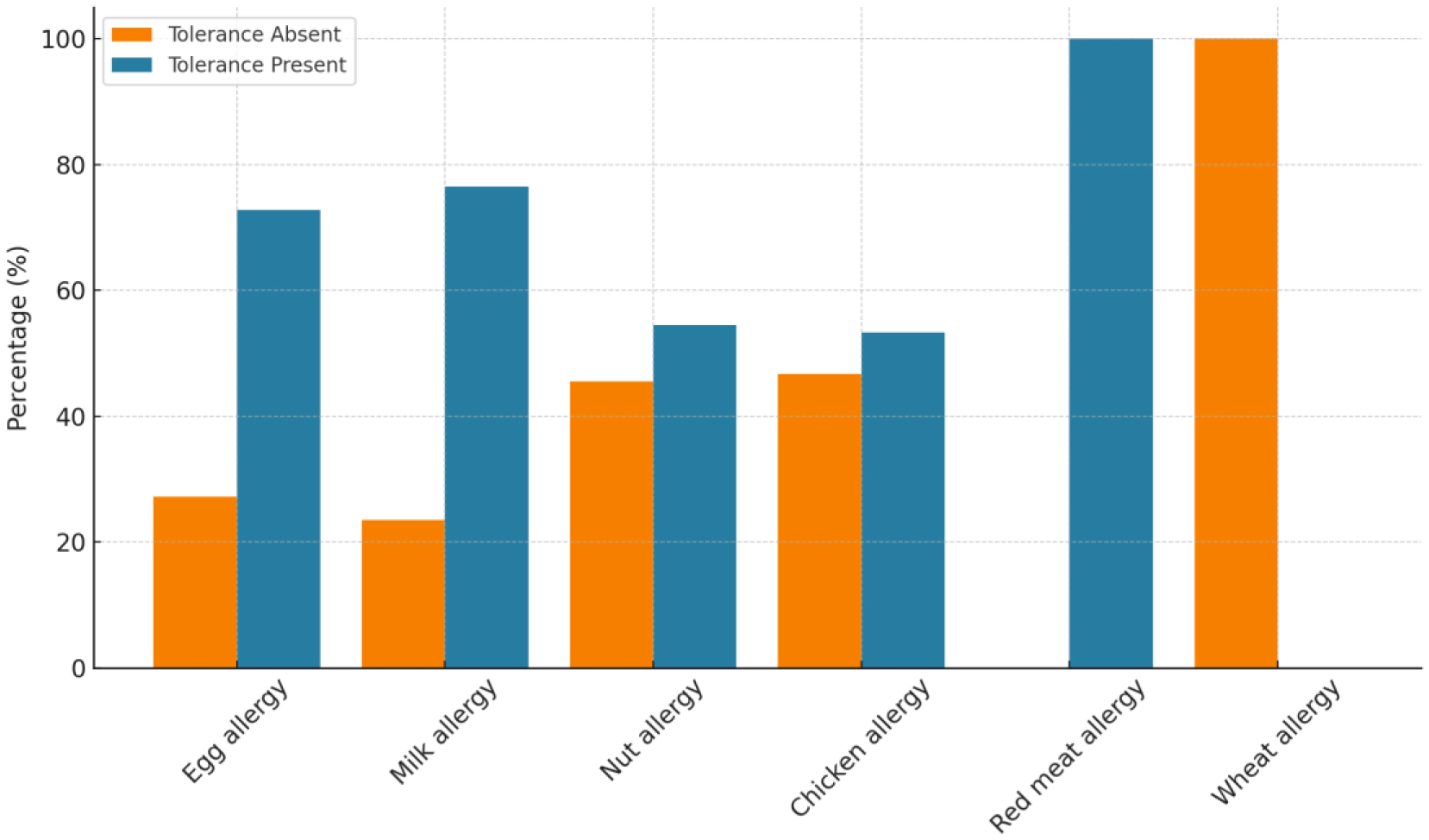
Objective: Food allergies, an immune reaction to food, affects 2–8% of children in developed countries, thereby presenting with symptoms ranging from anaphylaxis to gastrointestinal issues. This study explores the clinical and tolerance development aspects of pediatric food allergy cases at our clinic. Methods: This retrospective study included 187 pediatric patients with diagnosed food allergies from a pediatric allergy and immunology outpatient clinic at a training and research hospital. The patient files were retrospectively analyzed based on symptoms, improvements upon food removal from diets, food-specific IgE measurements, and skin prick tests. Results: This study included 187 pediatric patients diagnosed with food allergies, which were predominantly affected by eggs (66.8%) and cow's milk (54.5%). Tolerance developed in 73.3% of patients, with no significant differences based on age, gender, or comorbidities. Most patients with egg (72.8%) and milk (76.5%) allergies eventually developed a tolerance. While tolerance developed in 31.4% (n = 43) of patients with multiple allergies, tolerance developed in 68.6% (n = 94) of patients with an allergy to a single food. Conclusions: Our study of 187 pediatric patients highlighted egg and cow's milk as predominant allergens, with onsets typically in infancy. Tolerance developed in 73.3% of patients, with multiple allergies hindering tolerance acquisition. The median ages for tolerance were 12 months for cow's milk and 13 months for egg allergies, which indicates a relatively early resolution. The development of tolerance was found to be lower in patients with multiple food allergies than in patients with a single food allergy.

Conflict of interest

The authors declare that there is no conflict of interest in the preparation and publication of this article.

Author contributions

Conceptualization, S.Ç., M.Y.Ö. and U.A.; methodology, M.Y.Ö., Z.M.A., U.A.; validation, M.Y.Ö. and S.Ç.; formal analysis, S.Ç., U.A.; investigation, M.Y.Ö. and U.A.; resources, M.Y.Ö., S.Ç., and U.A.; data curation, S.Ç. and Z.M.A.; writing—original draft preparation, Z.M.A., S.Ç. and U.A.; writing—review and editing, M.Y.Ö. and S.Ç.; visualization, Z.M.A. and U.A.; supervision, M.Y.Ö and S.Ç. All authors have read and agreed to the published version of the manuscript.

References

[1]	Novak-Wegrzyn A, Burks AW, Sampson HA (2014) Reactions to food. Middleton's Allergy Principles and Practice . Philadelphia: Saunders Elsevier 1310-1339. https://doi.org/10.1016/B978-0-323-08593-9.00082-6
[2]	Sicherer SH, Sampson HA (2014) Food allergy: Epidemiology, pathogenesis, diagnosis, and treatment. J Allergy Clin Immunol 133: 291-307. https://doi.org/10.1016/j.jaci.2013.11.020
[3]	Bock SA, Sampson HA (2016) Evaluation of food allergy. Pediatric Allergy Principles and Practice . Philadelphia: Saunders Elsevier 371-376. https://doi.org/10.1016/B978-0-323-29875-9.00041-0
[4]	Burks W, Tang M, Sicherer S, et al. (2012) ICON: Food allergy. J Allergy Clin Immunol 129: 906-920. https://doi.org/10.1016/j.jaci.2012.02.001
[5]	Sicherer SH, Sampson HA (2010) Food allergy. J Allergy Clin Immunol 125: 116-125. https://doi.org/10.1016/j.jaci.2009.08.028
[6]	Ebisawa M, Ito K, Fujisawa T (2017) Japanese guidelines for food allergy 2017. Allergol Int 66: 248-264. https://doi.org/10.1016/j.alit.2017.02.001
[7]	Labrosse R, Graham F, Caubewt JC (2020) Non-IgE-mediated gastrointestinal food allergies in children: An update. Nutrients 12: 2086. https://doi.org/10.3390/nu12072086
[8]	Kazmi W, Berin MC (2023) Oral tolerance and oral immunotherapy for food allergy: Evidence for common mechanisms?. Cell Immunol 383: 104650. https://doi.org/10.1016/j.cellimm.2022.104650
[9]	Sicherer SH (2011) Epidemiology of food allergy. J Allergy Clin Immunol 127: 594-602. https://doi.org/10.1016/j.jaci.2010.11.044
[10]	Abrams EM, Shaker M, Stukus D, et al. (2023) Updates in food allergy prevention in children. Pediatrics 152: e2023062836. https://doi.org/10.1542/peds.2023-062836
[11]	Perrier C, Corthesy B (2011) Gut permeability and food allergies. Clin Exp Allergy 41: 20-28. https://doi.org/10.1111/j.1365-2222.2010.03639.x
[12]	Cerutti A, Chen K, Chorny A (2011) Immunoglobulin responses at the mucosal interface. Annu Rev Immunol 29: 273-293. https://doi.org/10.1146/annurev-immunol-031210-101317
[13]	Vickery BP, Burks W (2010) Oral immunotherapy for food allergy. Cur Opin Pediatr 22: 765-770. https://doi.org/10.1097/MOP.0b013e32833f5fc0
[14]	Anagnostou K, Meyer R, Fox A, et al. (2015) The rapidly changing world of food allergy in children. F1000Prime Rep 7: 35. https://doi.org/10.12703/P7-35
[15]	Keet C, Wood RA (2019). Food allergy in children: Prevalence, natural history, and monitoring for resolution
[16]	Yavuz ST, Sahiner UM, Buyuktiryaki B, et al. (2011) Phenotypes of IgE-mediated food allergy in Turkish children. Allergy Asthma Proc 32: 47-55. https://doi.org/10.2500/aap.2011.32.3481
[17]	Can C, Altınel N, Bülbül L, et al. (2019) Clinical and laboratory characteristics of patients with food allergy: Single-center experience. Med Bull Sisli Etfal Hosp 53: 296-299. https://doi.org/10.14744/SEMB.2018.23911
[18]	Allen KJ, Koplin JJ (2012) The epidemiology of IgE-mediated food allergy and anaphylaxis. Immunol Allergy Clin North Am 32: 35-50. https://doi.org/10.1016/j.iac.2011.11.008
[19]	Prescott S, Allen KJ (2011) Food allergy: Riding the second wave of the allergy epidemic. Pediatr Allergy Immunol 22: 155-160. https://doi.org/10.1111/j.1399-3038.2011.01145.x
[20]	Lack G (2012) Update on risk factors for food allergy. J Allergy Clin Immunol 129: 1187-1197. https://doi.org/10.1016/j.jaci.2012.02.036
[21]	Ersözlü Y, Anıl H, Harmanci K (2023) Factors affecting tolerance development in children with food allergies. Osmangazi Tıp Dergisi 45: 79-87. https://doi.org/10.20515/otd.1138002
[22]	Matricardi PM, Kleine-Tebbe J, Hoffmann HJ, et al. (2016) EAACI molecular allergology User's guide. Pediatr Allergy Immunol 27: 1-250. https://doi.org/10.1111/pai.12563
[23]	Calamelli E, Liotti L, Beghetti I, et al. (2019) Component-resolved diagnosis in food allergies. Medicina 55: 498. https://doi.org/10.3390/medicina55080498
[24]	Sturm GJ, Kranzelbinder B, Sturm EM, et al. (2009) The basophil activation test in the diagnosis of allergy: Technical issues and critical factors. Allergy 64: 1319-1326. https://doi.org/10.1111/j.1398-9995.2009.02004.x
[25]	Licari A, D'Auria E, De Amici M, et al. (2023) The role of basophil activation test and component-resolved diagnostics in the workup of egg allergy in children at low risk for severe allergic reactions: A real-life study. Pediatr Allergy Immunol 34: e14012. https://doi.org/10.1111/pai.14012
[26]	Shek LP, Soderstrom L, Ahlstedt S, et al. (2004) Determination of food specific IgE levels over time can predict the development of tolerance in cow's milk and hen's egg allergy. J Allergy Clin Immunol 114: 387-391. https://doi.org/10.1016/j.jaci.2004.04.032
[27]	Sicherer SH, Wood RA, Vickery BP, et al. (2014) The natural history of egg allergy in an observational cohort. J Allergy Clin Immunol 133: 492-499. https://doi.org/10.1016/j.jaci.2013.12.1041
[28]	Chong KW, Goh SH, Saffari SE, et al. (2022) IgE-mediated cow's milk protein allergy in Singaporean children. Asian Pac J Allergy Immunol 40: 65-71. https://doi.org/10.12932/AP-180219-0496
[29]	Dias A, Santos A, Pinheiro JA (2010) Persistence of cow's milk allergy beyond two years of age. Allergol Immunopathol 38: 8-12. https://doi.org/10.1016/j.aller.2009.07.005
[30]	Savage JH, Matsui EC, Skripak JM, et al. (2007) The natural history of egg allergy. J Allergy Clin Immunol 120: 1413-1417. https://doi.org/10.1016/j.jaci.2007.09.040
[31]	Larche M, Akdis CA, Valenta R (2006) Immunological mechanisms of allergen-specific immunotherapy. Nat Rev Immunol 6: 761-771. https://doi.org/10.1038/nri1934
[32]	Blumchen K, Ulbricht H, Staden U, et al. (2010) Oral peanut immunotherapy in children with peanut anaphylaxis. J Allergy Clin Immunol 126: 83-91.e1. https://doi.org/10.1016/j.jaci.2010.04.030
[33]	Wood RA (2017) Oral ımmunotherapy for food allergy. J Investig Allergol Clin Immunol 27: 151-159. https://doi.org/10.18176/jiaci.0143
[34]	Chinthrajah RS, Hernandez JD, Boyd SD, et al. (2016) Molecular and cellular mechanisms of food allergy and food tolerance. J Allergy Clin Immunol 137: 984-997. https://doi.org/10.1016/j.jaci.2016.02.004
[35]	Burks AW, Jones SM, Wood RA, et al. (2012) Oral immunotherapy for treatment of egg allergy in children. N Engl J Med 367: 233-243. https://doi.org/10.1056/NEJMoa1200435

Reader Comments

Your name:*

Email:*
© 2025 the Author(s), licensee AIMS Press. This is an open access article distributed under the terms of the Creative Commons Attribution License (http://creativecommons.org/licenses/by/4.0)