In this study, we present a rare case of familial amyloidosis polyneuropathy (FAP) caused by a novel mutation in the transthyretin protein (TTR) gene. A 40-year-old female patient presented with a complaint of numbness and weakness in both lower limbs that had persisted for a period of 18 months, accompanied by intermittent diarrhea. An analysis of her family history revealed that her father had succumbed to an instance of unexplained heart failure, while one of her siblings exhibited neurological symptoms of a comparable nature. A physical examination was conducted, which revealed sensory loss of distal symmetry, diminished tendon reflexes, and significant autonomic dysfunction. The skin biopsy revealed the presence of amyloid material deposits. Whole-exome sequencing revealed a novel mutation (c.179A>C, p.Thr60Pro), which replaces threonine with a proline at position 60 in the TTR gene. Subsequent screening revealed that other relatives carrying the same mutation also exhibited similar symptoms, thereby supporting the association between this mutation and FAP. This case underscores the significance of identifying novel TTR gene mutations, offers a novel perspective on the understanding of FAP, and posits that an early diagnosis and intervention are pivotal to enhance the prognosis.
Citation: Guoyan Chen, Jing Gao, Ziyao Li, Jine He. Familial exploration: A novel association of Thr 60Pro mutations in the Transthyretin gene with familial amyloidosis polyneuropathy[J]. AIMS Allergy and Immunology, 2025, 9(2): 89-97. doi: 10.3934/Allergy.2025006
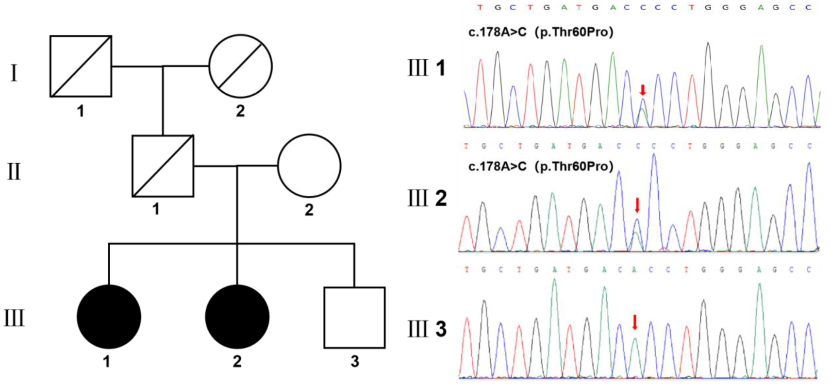
In this study, we present a rare case of familial amyloidosis polyneuropathy (FAP) caused by a novel mutation in the transthyretin protein (TTR) gene. A 40-year-old female patient presented with a complaint of numbness and weakness in both lower limbs that had persisted for a period of 18 months, accompanied by intermittent diarrhea. An analysis of her family history revealed that her father had succumbed to an instance of unexplained heart failure, while one of her siblings exhibited neurological symptoms of a comparable nature. A physical examination was conducted, which revealed sensory loss of distal symmetry, diminished tendon reflexes, and significant autonomic dysfunction. The skin biopsy revealed the presence of amyloid material deposits. Whole-exome sequencing revealed a novel mutation (c.179A>C, p.Thr60Pro), which replaces threonine with a proline at position 60 in the TTR gene. Subsequent screening revealed that other relatives carrying the same mutation also exhibited similar symptoms, thereby supporting the association between this mutation and FAP. This case underscores the significance of identifying novel TTR gene mutations, offers a novel perspective on the understanding of FAP, and posits that an early diagnosis and intervention are pivotal to enhance the prognosis.

| [1] | Adams D, Ando Y, Beirao JM, et al. (2021) Expert consensus recommendations to improve diagnosis of ATTR amyloidosis with polyneuropathy. J Neurol 268: 2109-2122. https://doi.org/10.1007/s00415-019-09688-0 |
| [2] | Andrade C (1952) A peculiar form of peripheral neuropathy; familiar atypical generalized amyloidosis with special involvement of the peripheral nerves. Brain 75: 408-427. https://doi.org/10.1093/brain/75.3.408 |
| [3] | Araki S, Mawatari S, Ohta M, et al. (1968) Polyneuritic amyloidosis in a Japanese family. Arch Neurol 18: 593-602. https://doi.org/10.1001/archneur.1968.00470360015001 |
| [4] | Andersson R (1976) Familial amyloidosis with polyneuropathy. A clinical study based on patients living in northern Sweden. Acta Med Scand Suppl 590: 1-64. |
| [5] | Lai Z, Colon W, Kelly JW (1996) The acid-mediated denaturation pathway of transthyretin yields a conformational intermediate that can self-assemble into amyloid. Biochemistry 35: 6470-6482. https://doi.org/10.1021/bi952501g |
| [6] | Saraiva MJ (2001) Transthyretin mutations in hyperthyroxinemia and amyloid diseases. Hum Mutat 17: 493-503. https://doi.org/10.1002/humu.1132 |
| [7] | Merlini G, Bellotti V (2003) Molecular mechanisms of amyloidosis. N Engl J Med 349: 583-596. https://doi.org/10.1056/NEJMra023144 |
| [8] | Araki S, Ando Y (2010) Transthyretin-related familial amyloidotic polyneuropathy-Progress in Kumamoto, Japan (1967–2010). Proc Jpn Acad Ser B Phys Biol Sci 86: 694-706. https://doi.org/10.2183/pjab.86.694 |
| [9] | Plante-Bordeneuve V, Lalu T, Misrahi M, et al. (1998) Genotypic-phenotypic variations in a series of 65 patients with familial amyloid polyneuropathy. Neurology 51: 708-714. https://doi.org/10.1212/wnl.51.3.708 |
| [10] | Ikeda S, Takei Y, Tokuda T, et al. (2003) Clinical and pathological findings of non-Val30Met TTR type familial amyloid polyneuropathy in Japan. Amyloid 10: 39-47. |
| [11] | Suhr OB, Lindqvist P, Olofsson BO, et al. (2006) Myocardial hypertrophy and function are related to age at onset in familial amyloidotic polyneuropathy. Amyloid 13: 154-159. https://doi.org/10.1080/13506120600876849 |
| [12] | Ando E, Ando Y, Okamura R, et al. (1997) Ocular manifestations of familial amyloidotic polyneuropathy type I: Long-term follow up. Br J Ophthalmol 81: 295-298. https://doi.org/10.1136/bjo.81.4.295 |
| [13] | Lobato L, Beirao I, Silva M, et al. (2004) End-stage renal disease and dialysis in hereditary amyloidosis TTR V30M: Presentation, survival and prognostic factors. Amyloid 11: 27-37. https://doi.org/10.1080/13506120410001673884 |
| [14] | Mariani LL, Lozeron P, Theaudin M, et al. (2015) Genotype-phenotype correlation and course of transthyretin familial amyloid polyneuropathies in France. Ann Neurol 78: 901-916. https://doi.org/10.1002/ana.24519 |
| [15] | Koike H, Tanaka F, Hashimoto R, et al. (2012) Natural history of transthyretin Val30Met familial amyloid polyneuropathy: Analysis of late-onset cases from non-endemic areas. J Neurol Neurosurg Psychiatry 83: 152-158. https://doi.org/10.1136/jnnp-2011-301299 |
| [16] | England JD, Gronseth GS, Franklin G, et al. (2009) Practice Parameter: Evaluation of distal symmetric polyneuropathy: Role of autonomic testing, nerve biopsy, and skin biops. Neurology 72: 177-184. https://doi.org/10.1212/01.wnl.0000336345.70511.0f |
| [17] | Westermark P (1995) Diagnosing amyloidosis. Scand J Rheumatol 24: 327-329. https://doi.org/10.3109/03009749509095175 |
| [18] | Smith LM, Sanders JZ, Kaiser RJ, et al. (1986) Fluorescence detection in automated DNA sequence analysis. Nature 321: 674-679. https://doi.org/10.1038/321674a0 |
| [19] | Conceicao I, Gonzalez-Duarte A, Obici L, et al. (2016) “Red-flag symptom” clusters in transthyretin familial amyloid polyneuropathy. J Peripher Nerv Syst 21: 5-9. https://doi.org/10.1111/jns.12153 |
| [20] | Di Stefano V, Lupica A, Alonge P, et al. (2024) Genetic screening for hereditary transthyretin amyloidosis with polyneuropathy in western Sicily: Two years of experience in a neurological clinic. Eur J Neurol 31: e16065. https://doi.org/10.1111/ene.16065 |
| [21] | Ericzon BG, Wilczek HE, Larsson M, et al. (2015) Liver transplantation for hereditary transthyretin amyloidosis: After 20 years still the best therapeutic alternative?. Transplantation 99: 1847-1854. https://doi.org/10.1097/TP.0000000000000574 |
| [22] | Waddington Cruz M, Amass L, Keohane D, et al. (2016) Early intervention with tafamidis provides long-term (5.5-year) delay of neurologic progression in transthyretin hereditary amyloid polyneuropathy. Amyloid 23: 178-183. https://doi.org/10.1080/13506129.2016.1207163 |
| [23] | Berk JL, Suhr OB, Obici L, et al. (2013) Repurposing diflunisal for familial amyloid polyneuropathy: A randomized clinical trial. JAMA 310: 2658-2667. https://doi.org/10.1001/jama.2013.283815 |
| [24] | Maurer MS, Schwartz JH, Gundapaneni B, et al. (2018) Tafamidis treatment for patients with transthyretin amyloid cardiomyopathy. N Engl J Med 379: 1007-1016. https://doi.org/10.1056/NEJMoa1805689 |
| [25] | Di Stefano V, Guaraldi P, Romano A, et al. (2025) Patisiran in ATTRv amyloidosis with polyneuropathy: “PatisiranItaly” multicenter observational study. J Neurol 272: 209. https://doi.org/10.1007/s00415-025-12950-3 |
| [26] | Ackermann EJ, Guo S, Benson MD, et al. (2016) Suppressing transthyretin production in mice, monkeys and humans using 2nd-Generation antisense oligonucleotides. Amyloid 23: 148-157. https://doi.org/10.1080/13506129.2016.1191458 |
| [27] | Richards DB, Cookson LM, Berges AC, et al. (2015) Therapeutic clearance of amyloid by antibodies to serum amyloid P component. N Engl J Med 373: 1106-1114. https://doi.org/10.1056/NEJMoa1504942 |
Figures(1)

Guoyan Chen, Jing Gao, Ziyao Li, Jine He. Familial exploration: A novel association of Thr 60Pro mutations in the Transthyretin gene with familial amyloidosis polyneuropathy[J]. AIMS Allergy and Immunology, 2025, 9(2): 89-97. doi: 10.3934/Allergy.2025006


 DownLoad: