Antibody profiling reveals gender differences in response to SARS-COVID-2 infection

Lia Tsverava; Nazibrola Chitadze; Gvantsa Chanturia; Merab Kekelidze; David Dzneladze; Paata Imnadze; Amiran Gamkrelidze; Vincenzo Lagani; Zaza Khuchua; Revaz Solomonia; Lia Tsverava; Nazibrola Chitadze; Gvantsa Chanturia; Merab Kekelidze; David Dzneladze; Paata Imnadze; Amiran Gamkrelidze; Vincenzo Lagani; Zaza Khuchua; Revaz Solomonia

doi:10.3934/Allergy.2022002

AIMS Allergy and Immunology

2022, Volume 6, Issue 1: 6-13. doi: 10.3934/Allergy.2022002

Previous Article Next Article

Research article Topical Sections

Antibody profiling reveals gender differences in response to SARS-COVID-2 infection

1.
Institute of Chemical Biology, Ilia State University, Tbilisi, Georgia
2.
I.Beritashvili Center of Experimental Biomedicine, Tbilisi, Georgia
3.
National Center for Disease Control, Tbilisi, Georgia
4.
Sechenov University, Department of Biochemistry, Moscow, Russia
5.
Biological and Environmental Sciences and Engineering Division (BESE), King Abdullah University of Science and Technology KAUST, Thuwal, Saudi Arabia

Received: 29 October 2021 Revised: 29 November 2021 Accepted: 20 December 2021 Published: 10 January 2022

The recent emergence of the novel severe acute respiratory syndrome coronavirus 2 (SARS-CoV-2) has led to an ongoing global COVID-19 pandemic and public health crisis. Detailed study of human immune response to SARS-CoV-2 infection is the important topic for a successful treatment of this disease. Our study was aimed to characterize immune response on the level of antibody profiling in convalescent plasma of patients in Georgia. Antibodies against the following SARS-CoV-2 proteins were studied: nucleocapsid and various regions of spike (S) protein: S1, S2 and receptor binding domain (RBD). Convalescent plasma of patients 6–8 weeks after initial confirmation of SARS-CoV-2 infection were tested. Nearly 80% out of 162 patients studied showed presence of antibodies against nucleocapsid protein. The antibody response to three fragments of S protein was significantly less and varied in the range of 20–30%. Significantly more females as compared to males were producing antibodies against S1 fragment, whereas the difference between genders by the antibodies against nucleocapsid protein and RBD was statistically significant only by one-tailed Fisher exact test. There were no differences between the males and females by antibodies against S2 fragment. Thus, immune response against some viral antigens is stronger in females and we suggest that it could be one of the factors of less female fatality after SARS-CoV-2 infection.
- SARS-CoV-2,
- immune response,
- nucleocapside protein,
- S protein,
- gender differences
Citation: Lia Tsverava, Nazibrola Chitadze, Gvantsa Chanturia, Merab Kekelidze, David Dzneladze, Paata Imnadze, Amiran Gamkrelidze, Vincenzo Lagani, Zaza Khuchua, Revaz Solomonia. Antibody profiling reveals gender differences in response to SARS-COVID-2 infection[J]. AIMS Allergy and Immunology, 2022, 6(1): 6-13. doi: 10.3934/Allergy.2022002

Related Papers:

Abstract

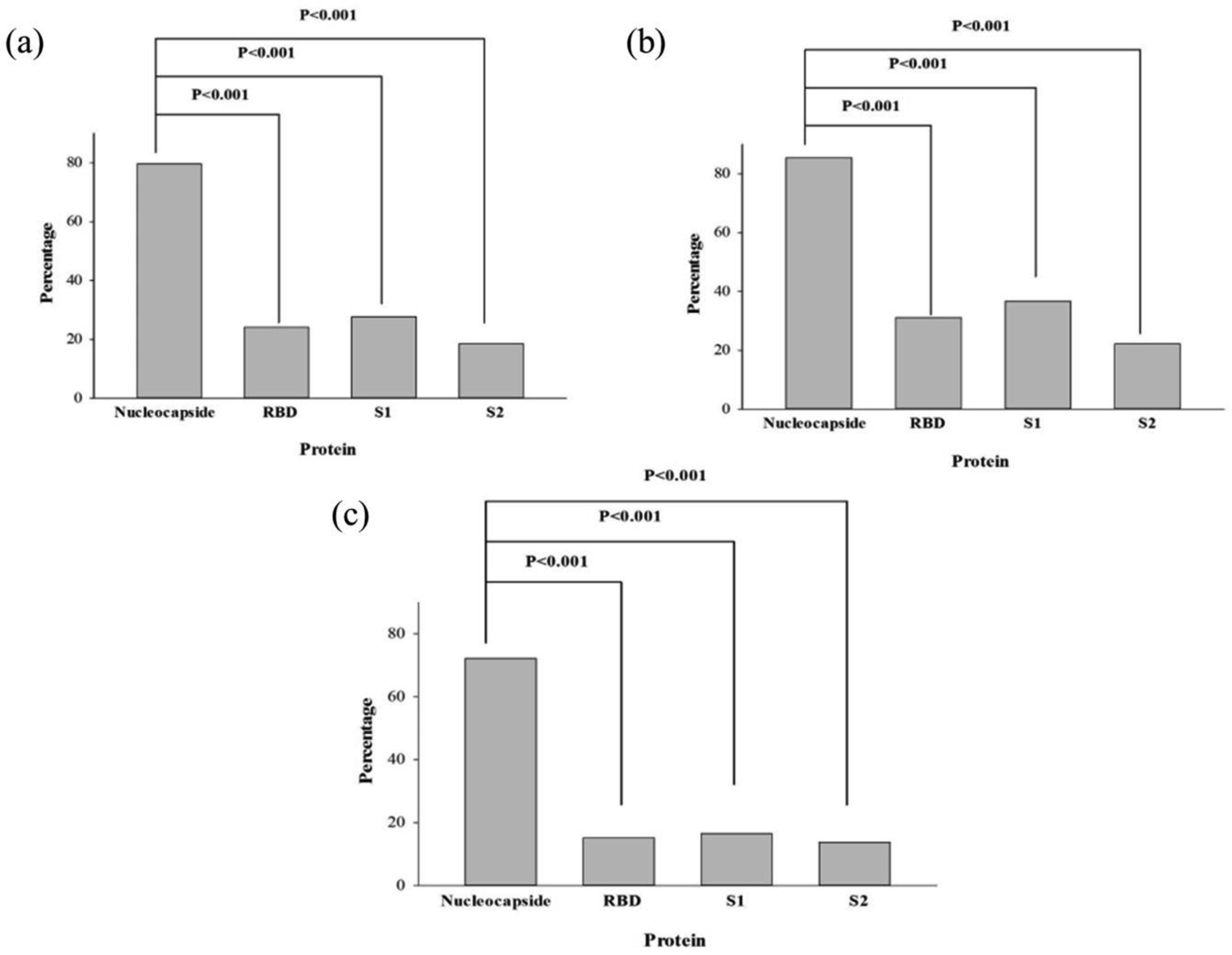
The recent emergence of the novel severe acute respiratory syndrome coronavirus 2 (SARS-CoV-2) has led to an ongoing global COVID-19 pandemic and public health crisis. Detailed study of human immune response to SARS-CoV-2 infection is the important topic for a successful treatment of this disease. Our study was aimed to characterize immune response on the level of antibody profiling in convalescent plasma of patients in Georgia. Antibodies against the following SARS-CoV-2 proteins were studied: nucleocapsid and various regions of spike (S) protein: S1, S2 and receptor binding domain (RBD). Convalescent plasma of patients 6–8 weeks after initial confirmation of SARS-CoV-2 infection were tested. Nearly 80% out of 162 patients studied showed presence of antibodies against nucleocapsid protein. The antibody response to three fragments of S protein was significantly less and varied in the range of 20–30%. Significantly more females as compared to males were producing antibodies against S1 fragment, whereas the difference between genders by the antibodies against nucleocapsid protein and RBD was statistically significant only by one-tailed Fisher exact test. There were no differences between the males and females by antibodies against S2 fragment. Thus, immune response against some viral antigens is stronger in females and we suggest that it could be one of the factors of less female fatality after SARS-CoV-2 infection.

Acknowledgments

The work was supported by National Center for Disease Control, Tbilisi, Georgia and Ilia State University, Tbilisi, Georgia.

Conflict of interest

All authors declare no conflicts of interest in this paper.

References

[1]	Dehingia N, Raj A (2021) Sex differences in COVID-19 case fatality: do we know enough? Lancet Glob Health 9: e14-e15. https://doi.org/10.1016/S2214-109X(20)30464-2. doi: 10.1016/S2214-109X(20)30464-2
[2]	Takahashi T, Ellingson MK, Wong P, et al. (2020) Sex differences in immune responses that underlie COVID-19 disease outcomes. Nature 588: 315-320. https://doi.org/10.1038/s41586-020-2700-3. doi: 10.1038/s41586-020-2700-3
[3]	Kadam SB, Sukhramani GS, Bishnoi P, et al. (2021) SARS-CoV-2, the pandemic coronavirus: Molecular and structural insights. J Basic Microbiol 61: 180-202. https://doi.org/10.1002/jobm.202000537. doi: 10.1002/jobm.202000537
[4]	Troyano-Hernáez P, Reinosa R, Holguín Á (2021) Evolution of SARS-CoV-2 envelope, membrane, nucleocapsid, and spike structural proteins from the beginning of the pandemic to September 2020: A global and regional approach by epidemiological week. Viruses 13: 243https://doi.org/10.3390/v13020243. doi: 10.3390/v13020243
[5]	Leung DTM, Tam FCH, Ma CH, et al. (2004) Antibody response of patients with severe acute respiratory syndrome (SARS) targets the viral nucleocapsid. J Infect Dis 190: 379-386. https://doi.org/10.1086/422040. doi: 10.1086/422040
[6]	Klasse PJ, Sanders RW, Cerutti A, et al. (2012) How can HIV-type-1-Env immunogenicity be improved to facilitate antibody-based vaccine development? Aids Res Hum Retrov 28: 1-15. https://doi.org/10.1089/aid.2011.0053. doi: 10.1089/aid.2011.0053
[7]	Nozadze M, Zhgenti E, Meparishvili M, et al. (2015) Comparative proteomic studies of yersinia pestis strains isolated from natural foci in the Republic of Georgia. Front Public Health 3: 239https://doi.org/10.3389/fpubh.2015.00239. doi: 10.3389/fpubh.2015.00239
[8]	R Core Team R: A Language and Environment for Statistical Computing. R Foundation for Statistical Computing (2021) .Available from: https://www.R-project.org/.
[9]	Hoffmann M, Kleine-Weber H, Schroeder S, et al. (2020) SARS-CoV-2 cell entry depends on ACE2 and TMPRSS2 and is blocked by a clinically proven protease inhibitor. Cell 181: 271-280. https://doi.org/10.1016/j.cell.2020.02.052. doi: 10.1016/j.cell.2020.02.052
[10]	Gadi N, Wu SC, Spihlman AP, et al. (2020) What's sex got to do with COVID-19? Gender-based differences in the host immune response to coronaviruses. Front Immunol 11: 2147https://doi.org/10.3389/fimmu.2020.02147. doi: 10.3389/fimmu.2020.02147
[11]	Channappanavar R, Fett C, Mack M, et al. (2017) Sex-based differences in susceptibility to severe acute respiratory syndrome coronavirus infection. J Immunol 198: 4046-4053. https://doi.org/10.4049/jimmunol.1601896. doi: 10.4049/jimmunol.1601896
[12]	Moulton VR (2018) Sex hormones in acquired immunity and autoimmune disease. Front Immunol 9: 2279https://doi.org/10.3389/fimmu.2018.02279. doi: 10.3389/fimmu.2018.02279
[13]	Schurz H, Salie M, Tromp G, et al. (2019) The X chromosome and sex-specific effects in infectious disease susceptibility. Hum Genomics 13: 2https://doi.org/10.1186/s40246-018-0185-z. doi: 10.1186/s40246-018-0185-z
[14]	Chamekh M, Casimir G (2019) Sexual dimorphism of the immune inflammatory response in infectious and non-infectious diseases. Front Immunol 10: 107https://doi.org/10.3389/fimmu.2019.00107. doi: 10.3389/fimmu.2019.00107
[15]	Wang J, Syrett CM, Kramer MC, et al. (2016) Unusual maintenance of X chromosome inactivation predisposes female lymphocytes for increased expression from the inactive X. P Natl Acad Sci USA 113: E2029-E2038. https://doi.org/10.1073/pnas.1520113113. doi: 10.1073/pnas.1520113113

Reader Comments

your name:*

Email:*
© 2022 the Author(s), licensee AIMS Press. This is an open access article distributed under the terms of the Creative Commons Attribution License (http://creativecommons.org/licenses/by/4.0)