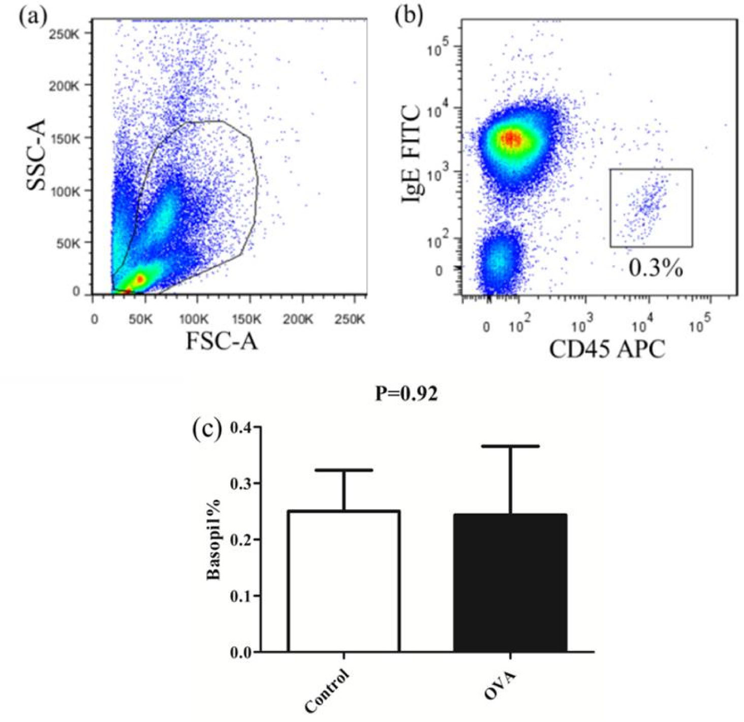
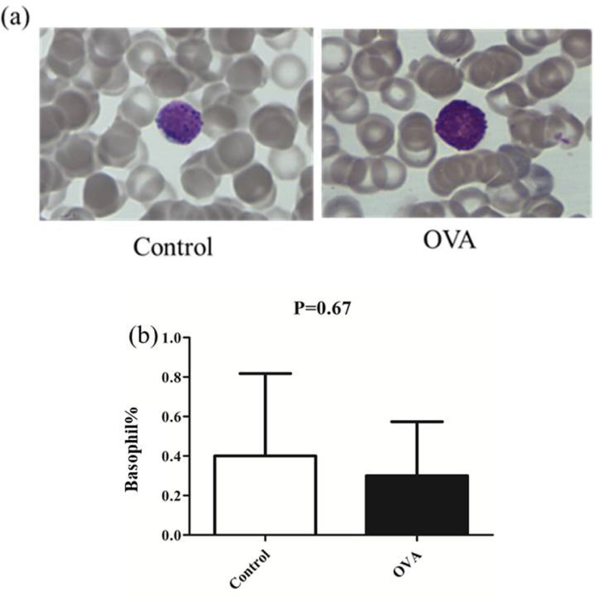
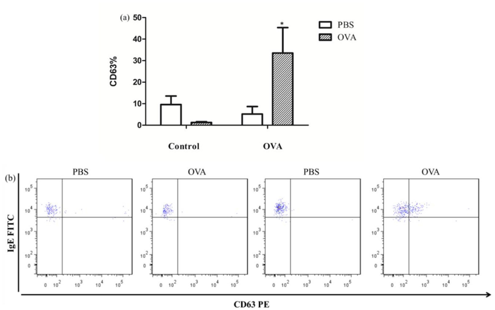
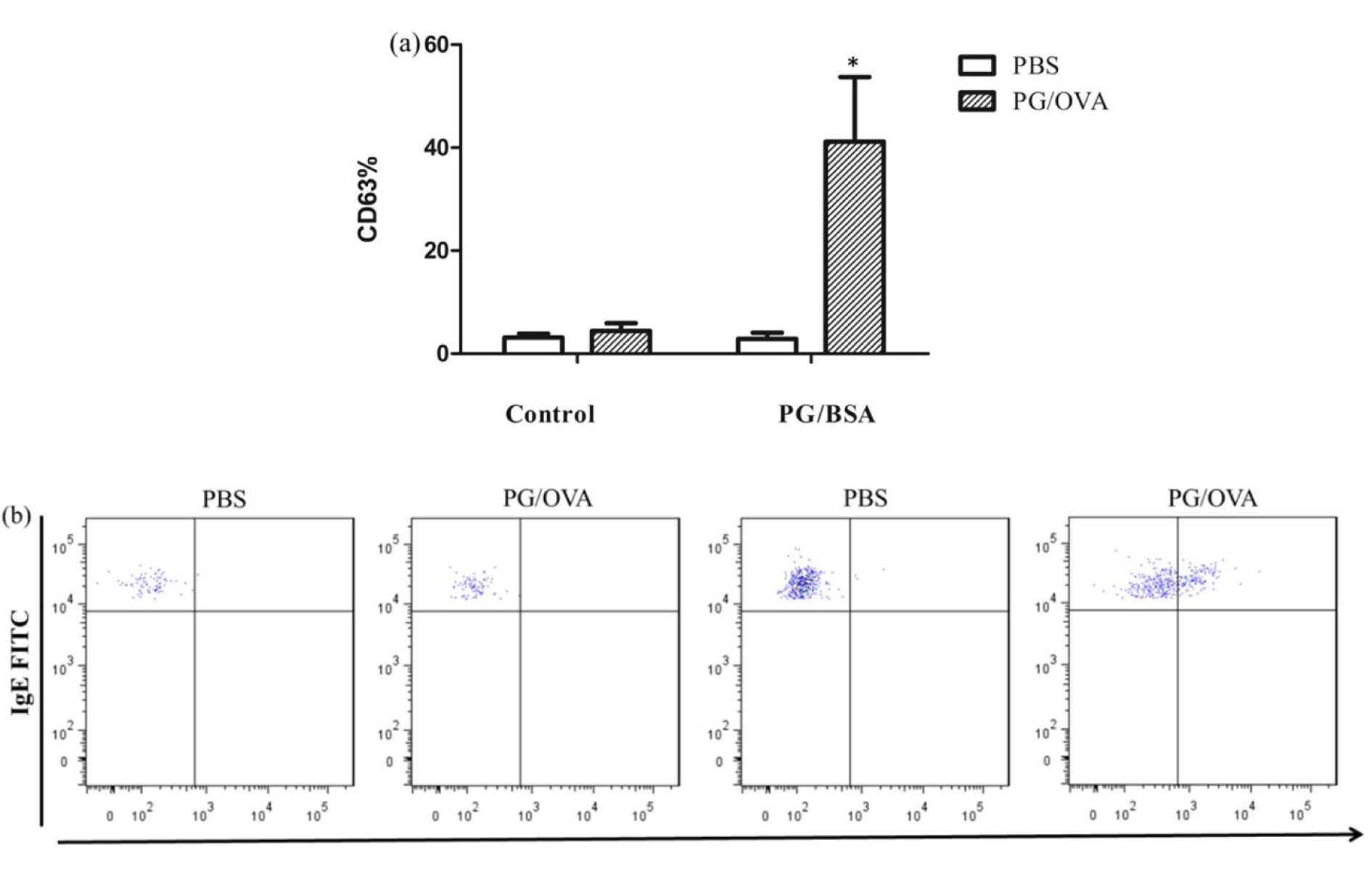
Allergies induced by low molecular weight compounds (LMWCs) have become a major problem in clinical medication. Effective preclinical prediction of sensitization can solve this problem; however, there are currently no reliable methods to predict sensitization, and it is necessary to establish a more effective model. The basophil activation test (BAT) has been widely used clinically to diagnose and research allergic diseases with high sensitivity. The purpose of this study was to detect the expression of CD63 in basophils in OVA-sensitized brown Norway (BN) rats, establishing a model for the BAT to assess the sensitization of the low molecular weight compound PG. The number of basophils in rats was detected by flow cytometry and blood smear analysis. The peripheral blood of OVA-sensitized rats was incubated with OVA, and the increase in CD63 on basophils was greater than that with PBS in vitro. After penicillin G-conjugated OVA (PG/OVA) was incubated with the peripheral blood of penicillin G-conjugated BSA (PG/BSA)-sensitized rats, the expression of CD63 on basophils was significantly higher than that with PBS. The basophils in the sensitized rats were again exposed to the same antigen in vitro, and flow cytometry detected a significant increase in CD63, demonstrating that the rat BAT model was successfully built, and it can be used to evaluate the potential sensitization of low molecular weight compounds.
Citation: Yanru Guo, Rong Sun, Wei Li, Zhaohua Liu. Establishment of a basophil activation test in BN rats[J]. AIMS Allergy and Immunology, 2020, 4(2): 20-31. doi: 10.3934/Allergy.2020003
Allergies induced by low molecular weight compounds (LMWCs) have become a major problem in clinical medication. Effective preclinical prediction of sensitization can solve this problem; however, there are currently no reliable methods to predict sensitization, and it is necessary to establish a more effective model. The basophil activation test (BAT) has been widely used clinically to diagnose and research allergic diseases with high sensitivity. The purpose of this study was to detect the expression of CD63 in basophils in OVA-sensitized brown Norway (BN) rats, establishing a model for the BAT to assess the sensitization of the low molecular weight compound PG. The number of basophils in rats was detected by flow cytometry and blood smear analysis. The peripheral blood of OVA-sensitized rats was incubated with OVA, and the increase in CD63 on basophils was greater than that with PBS in vitro. After penicillin G-conjugated OVA (PG/OVA) was incubated with the peripheral blood of penicillin G-conjugated BSA (PG/BSA)-sensitized rats, the expression of CD63 on basophils was significantly higher than that with PBS. The basophils in the sensitized rats were again exposed to the same antigen in vitro, and flow cytometry detected a significant increase in CD63, demonstrating that the rat BAT model was successfully built, and it can be used to evaluate the potential sensitization of low molecular weight compounds.

| [1] |
Minegaki Y, Higashida Y, Ogawa M, et al. (2013) Drug–induced hypersensitivity syndrome complicated with concurrent fulminant type 1 diabetes mellitus and Hashimoto's thyroiditis. Int J Dermatol 52: 355-357. doi: 10.1111/j.1365-4632.2011.05213.x

|
| [2] |
Muraro A, Lemanske RF, Castells M, et al. (2017) Precision medicine in allergic disease—food allergy, drug allergy, and anaphylaxis—PRACTALL document of the European Academy of Allergy and Clinical Immunology and the American Academy of Allergy, Asthma and Immunology. Allergy 72: 1006-1021. doi: 10.1111/all.13132
|
| [3] |
Hoffmann HJ, Santos AF, Mayorga C, et al. (2015) The clinical utility of basophil activation testing in diagnosis and monitoring of allergic disease. Allergy 70: 1393-1405. doi: 10.1111/all.12698
|
| [4] |
Larsen LF, Juel–Berg N, Hansen KS, et al. (2018) A comparative study on basophil activation test, histamine release assay, and passive sensitization histamine release assay in the diagnosis of peanut allergy. Allergy 73: 137-144. doi: 10.1111/all.13243
|
| [5] |
Venkatesan N, Siddiqui S, Jo T, et al. (2012) Allergen-induced airway remodeling in brown norway rats: structural and metabolic changes in glycosaminoglycans. Am J Resp Cell Mol 46: 96-105. doi: 10.1165/rcmb.2011-0014OC
|
| [6] | Guo SS, Wang YZ, Zhang Y, et al. (2009) Allergic response of Shuanghuanglian injection in BN rats and guinea pigs. Chinese J Pharmacol Toxicol 23: 128-133. |
| [7] |
Sudheer PS, Hall JE, Read GF, et al. (2005) Flow cytometric investigation of peri–anaesthetic anaphylaxis using CD63 and CD203c. Anaesthesia 60: 251-256. doi: 10.1111/j.1365-2044.2004.04086.x
|
| [8] |
Nagao K, Yokoro K, Aaronson SA (1981) Continuous lines of basophil/mast cells derived from normal mouse bone marrow. Science 212: 333-335. doi: 10.1126/science.7209531
|
| [9] | Guo L, Chen J, Gu G, et al. (2008) A Novel Method for Enumeration of Basophiles in Peripheral Blood by Flow Cytometry. J Mod Lab Med 23: 91-93. |
| [10] |
Santos AF, Lack G (2016) Basophil activation test: food challenge in a test tube or specialist research tool? Clin Transl Allergy 6: 10. doi: 10.1186/s13601-016-0098-7
|
| [11] | Chomiciene A, Jurgauskiene L, Kowalski ML, et al. (2014) Serum induced CD63 and CD203c activation tests in chronic urticaria. Cent Eur J Med 9: 339-347. |
| [12] |
Giavina–Bianchi P, Galvão VR, Picard M, et al. (2017) Basophil activation test is a relevant biomarker of the outcome of rapid desensitization in platinum compounds–allergy. J Allergy Clin Immunol Pract 5: 728-736. doi: 10.1016/j.jaip.2016.11.006
|
| [13] |
Kimber I, Betts CJ, Dearman RJ (2003) Assessment of the allergenic potential of proteins. Toxicol Lett 140: 297-302. doi: 10.1016/S0378-4274(03)00025-0
|
| [14] | Cooper AD, Balakrishnan K, McConnell HM (1981) Mobile haptens in liposomes stimulate serotonin release by rat basophil leukemia cells in the presence of specific immunoglobulin E. J Biol Chem 256: 9379-9381. |
| [15] |
Kane P, Holowka D, Baird B (1990) Characterization of model antigens composed of biotinylated haptens bound to avidin. Immunol Invest 19: 1-25. doi: 10.3109/08820139009042022
|
| [16] |
Cliquet P, Cox E, Van Dorpe C, et al. (2001) Generation of class–selective monoclonal antibodies against the penicillin group. J Agr Food Chem 49: 3349-3355. doi: 10.1021/jf001428k
|
| [17] |
Fernández TD, Torres MJ, Blanca–Lopez N, et al. (2009) Negativization rates of IgE radioimmunoassay and basophil activation test in immediate reactions to penicillins. Allergy 64: 242-248. doi: 10.1111/j.1398-9995.2008.01713.x
|
| [18] | Pan QJ, Liu Y, Fu N (2009) Research progress of basophils in allergy and immune response. Chinese J Immunol 25: 671-673. Available from: https://www.ixueshu.com/document/a0d7bb67273064f37d0e96385936a0fa318947a18e7f9386.html. |
| [19] |
Ebo DG, Sainte–Laudy J, Bridts CH, et al. (2006) Flow–assisted allergy diagnosis: current applications and future perspectives. Allergy 61: 1028-1039. doi: 10.1111/j.1398-9995.2006.01039.x
|
Figures(6)

Yanru Guo, Rong Sun, Wei Li, Zhaohua Liu. Establishment of a basophil activation test in BN rats[J]. AIMS Allergy and Immunology, 2020, 4(2): 20-31. doi: 10.3934/Allergy.2020003


 DownLoad: