Citation: Nikolai Pushkarev. A CAP for Healthy LivingMainstreaming Health into the EU Common Agricultural Policy
European Public Health Alliance (EPHA), 2015[J]. AIMS Public Health, 2015, 2(4): 844-887. doi: 10.3934/publichealth.2015.4.844

| [1] | Phil Hogan EU Commissioner for Agriculture (2015) Interview at the Forum for the Future of Agriculture by Views.eu, [online]. While using this quote EPHA however disagrees that the CAP should not be about farmers. |
| [2] | Tim Lang (2004) European agricultural policy: Is health the missing link? In: London School of Economics and Political Science, Eurohealth issue: Integrating Public Health with European food and agricultural policy. online. Of course the policy also aimed to provide economic security for the farming population, which is visible in the CAP's mission statement. |
| [3] | Also, in the past nutrient recommendation for protein intake, especially animal protein, was around twice as high as it is today, see for instance: J. Périssé (1981) Joint FAO/WHO/UNU Expert Consultation on Energy and Protein Requirements [online]. |
| [4] | WHO Europe (2015) European Health Report 2015. [online] |
| [5] | Art 168 Treaty on the Functioning of the European Union (TFEU). [online] |
| [6] | WHO Europe (2012) Action plan for implementation of the European strategy for the Prevention and Control of Noncommunicable Diseases 2012-2016, p. 5. [online] |
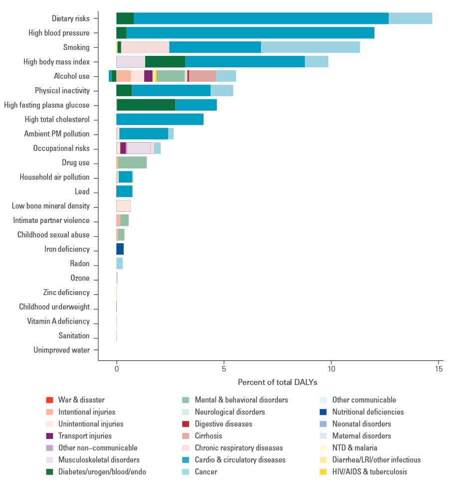
| [7] | Outcome of the “Global Burden of Disease” study (2013), a collaboration between seven leading international scientific institutes to systematically quantify the main causes of health loss. Institute for Health Metrics and Evaluation. University of Washington (2013) The global burden of disease. Generating evidence, guiding policy. European Union and European Free Trade Association Regional Edition. [online] |
| [8] | The Disability Adjusted Life Year (DALY) is a measure of overall disease burden expressed as the number of years lost due to ill-health, disability or early death. The measure combines mortality and disease into one indicator. |
| [9] | European Commission. Infographic: Tobacco in the EU. [online] |
| [10] | FAO (2012) Sustainable diets and biodiversity. Directions and solutions for policy research and action. Proceedings of International Scientific Symposium. [online] |
| [11] | Tim Lang et al. (2012) Ecological public health: the 21st century's big idea? The BMJ. [online] |
| [12] | Lancet Commission on planetary health (2015) Safeguarding human health in the Anthropocene epoch. The Lancet. [online] |
| [13] | Nick Watts et al. (2015) Health and climate change: policy responses to protect public health. The Lancet. [online] |
| [14] | National Nutrition Council of Finland (2014) Finnish Nutrition Recommendations 2014. [online] |
| [15] | Global Meat News (2015) Latest US dietary advice to avoid limiting meat. [online] |
| [16] | European Commission (2013) Overview of CAP Reform 2014-2020. [online] |
| [17] | OECD (2015) Focus on Health Spending. Health Statistics 2015. [online] |
| [18] | OECD iLibrary, Health at a Glance: Europe 2012. [online] |
| [19] | Vytenis Andriukaitis (16 July 2015) Speech outlining priorities for health until 2019 at European Policy Centre, [online] |
| [20] | Sophie Hawkesworth et al. (2010) Feeding the world healthily: the challenge of measuring the effects of agriculture on health. Philosophical Transactions B of The Royal Society. [online] |
| [21] | Schäfer Elinder (2003) Public health aspects of the EU Common Agricultural Policy. Developments and recommendations for change in four sectors: Fruit and vegetables, dairy, wine and tobacco. National Institute of Public Health, Sweden |
| [22] | Christopher Birt et al. (2007) A CAP on Health? The impact of the EU Common Agricultural Policy on public health. Faculty of Public Health. [online] |
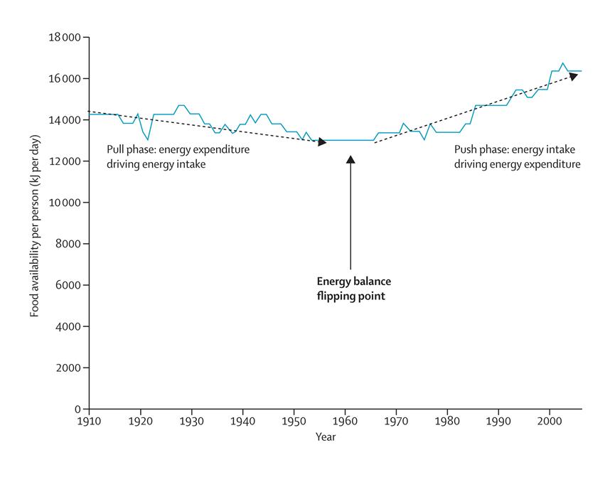
| [23] | Boyd Swinburn et al. (2011) The global obesity pandemic: shaped by global drivers and local environments. The Lancet. [online] |
| [24] | Stefanie Vandevijvere et al. (2015) Increased food energy supply as a major driver of the obesity epidemic: a global perspective. Bulletin of the World Health Organisation. [online] |
| [25] | Boyd Swinburn et al. (2009) Increased food energy supply is more than sufficient to explain the US epidemic of obesity. Am J Clin Nutr. [online] |
| [26] | P. Scarborough et al. (2011) Increased energy intake entirely accounts for increase in body weight in women but not in men in the UK between 1968 and 2000. Br J Nutr. [online] |
| [27] | T. Rawe et al. (2015) Cultivating equality: delivering just and sustainable food systems in a changing climate. CGIAR. [online] |
| [28] | Josef Schmidhuber (2007) The EU Diet - Evolution, Evaluation and Impacts of the CAP. FAO. [online] |
| [29] | Ralf Peters (2006) Roadblock to reform: the persistence of agricultural export subsidies. UNCTAD. [online] |
| [30] | Eurostat. Cross-country comparison of final consumption expenditures on food and housing in 2011. [online] |
| [31] | Franco Sassi (2010) Obesity and the Economics of Prevention - Fit not fat. OECD. [online] |
| [32] | D. Lakdawalla et al. (2002) The Growth of Obesity and Technological Change: A theoretical and Empirical Examination. National Bureau for Economic Research. Working Paper W8946. [online] |
| [33] | Alan Matthews (2015) Forum for the Future of Agriculture 2015 - Remarks on EU agricultural trade policy. CAPreform.eu. [online] |
| [34] | Corinna Hawkes et al. (2012) Linking agricultureal policies with obesity and noncommunicable diseases: A new perspective for a globalising world. Food Policy. [online] |
| [35] | A similar case was made by: The Netherlands Scientific Council for Government Policy (2014) Towards a food policy. English synopsis. [online] |
| [36] | WHO Europe (2000) The First Action Plan for Food and Nutrition Policy (2000-2005). [online] |
| [37] | EPHA (2010) Response to the “The Future of the Common Agricultural Policy” consultation. online. European Public Health & Agriculture Consortium (2011) Response to the “Reform of the CAP towards 2020 - impact assessment”. [online] |
| [38] | Olivier de Schutter (2014) Report of the Special Rapporteur on the right to food, Final report: The transformative potential of the right to food. UN. [online] |
| [39] | Regulation (EU) No 1307/2013 establishing rules for direct payments to farmers under support schemes within the framework of the common agricultural policy. [online] |
| [40] | Regulation (EU) No 1308/2013 establishing a common organisation of the markets in agricultural products. [online] |
| [41] | Regulation (EU) No 1305/2013 on support for rural development. [online] |
| [42] | Treaty on the European Union. online. Treaty on the Functioning of the European Union. [online] |
| [43] | Karen Lock et al. (2003) Health impact assessment of agriculture and food policies: lessons learnt from the Republic of Slovenia. Bulletin of the World Health Organisation. [online] |
| [44] | Vytenis Andriukaitis. EU Commissioner for Health (2015) Letter to the EU Ministers of Health. [online] |
| [45] | Scotch Whisky Association, the European Spirits Association and the Comité Européen des Entreprises Vins. |
| [46] | Scottish Court of Session (2013) Opinion by Lord Doherty. online. Judiciary of Scotland (2013) Petition for Judicial Review by Scotch Whisky Association & Others, [online] |
| [47] | Politico (2015) Health chief blasts alcohol lobbyists. [online] |
| [48] | Case C-333/14: Reference for a preliminary ruling from Court of Session, Scotland (United Kingdom) made on 8 July 2014 — The Scotch Whisky Association and others against The Lord Advocate, The Advocate General for Scotland. [online] |
| [49] | Opinion of Advocate General Yves Bot (2015) In the case: The Scotch Whisky Association and others against The Lord Advocate, The Advocate General for Scotland. [online] |
| [50] | WHO (2014) Global Status Report on Alcohol and Health 2014. [online] |
| [51] | OECD (2015) Tackling harmful alcohol use. online. OECD (2015) Policy Brief. Tackling harmful alcohol use, [online] |
| [52] | Giulia Meloni et al. (2012) The Political Economy of European Wine Regulation. Centre for Institutions and Economic Performance. Catholic University of Leuven. [online] |
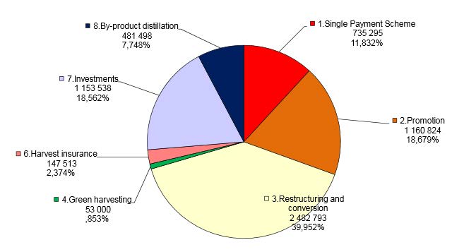
| [53] | European Commission (2006) Towards a sustainable European wine sector. [online] |
| [54] | European Court of Auditors (2014) Is the EU investment and promotion support to the wine sector well managed and are its results on the competitiveness of EU wines demonstrated?. [online] |
| [55] | European Court of Auditors (2012) The reform of the common organisation of the market in wine: progress to date. [online] |
| [56] | Article 63 CMO Regulation. Member States may also choose to authorise less, but it may not be 0% or lower. |
| [57] | European Court of Auditors (2014) Is the EU investment and promotion support to the wine sector well managed and are its results on the competitiveness of EU wines demonstrated? [online] |
| [58] | Article 39 CMO Regulation |
| [59] | Articles 45 to 52 of the CMO Regulation |
| [60] | Article 44 CMO Regulation referring to Annex VI |
| [61] | European Commission (2013) Wine CMO: First submission of financial table of the national support programme. [online]. Submissions were made under the previous CMO for wine, reviewed national envelopes are forthcoming. |
| [62] | Article 45 CMO Regulation |
| [63] | European Court of Auditors (2014) Is the EU investment and promotion support to the wine sector well managed and are its results on the competitiveness of EU wines demonstrated? [online] |
| [64] | Articles 50 and 51 CMO Regulation |
| [65] | European Court of Auditors (2014) Is the EU investment and promotion support to the wine sector well managed and are its results on the competitiveness of EU wines demonstrated? [online] |
| [66] | Articles 48 and 49 CMO Regulation |
| [67] | Articles 47 CMO Regulation |
| [68] | Articles 52 CMO Regulation |
| [69] | For more on the effects of the previous distillation support regimes: Schäfer Elinder (2003) Public health aspects of the EU Common Agricultural Policy. Developments and recommendations for change in four sectors: Fruit and vegetables, dairy, wine and tobacco. National Institute of Public Health, Sweden. |
| [70] | European Commission (2002) Ex-post evaluation of the CMO for wine, Chapter 5. Distillation. [online] |
| [71] | Article 46 CMO Regulation |
| [72] | European Court of Auditors (2012) The reform of the common organisation of the market in wine: progress to date. [online] |
| [73] | Giulia Meloni et al. (2015) L'Histoire se repete. Why the liberalization of the EU vineyard planting rights regime may require another French Revolution. Centre for Institutions and Economic Performance. Catholic University of Leuven. [online] |
| [74] | European Court of Auditors (2012) The reform of the common organisation of the market in wine: progress to date. [online] |
| [75] | Giulia Meloni et al. (2015) L'Histoire se repete. Why the liberalization of the EU vineyard planting rights regime may require another French Revolution. Centre for Institutions and Economic Performance. Catholic University of Leuven. [online] |
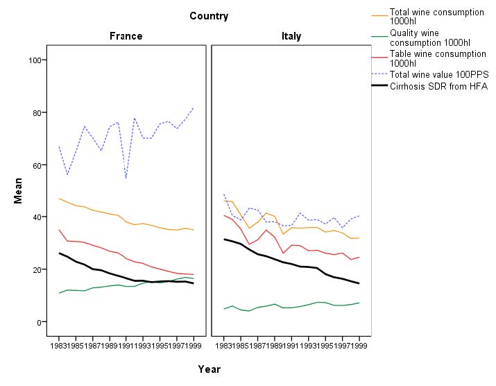
| [76] | Nick Sheron, University of Southampton, unpublished graph. Values are measured in Purchasing Power Standard (PPS) based on data provided by DG AGRI, Eurostat and the WHO HFA database and analysed in SPSS(48, 78). |
| [77] | The Brewers of Europe (2014) Beer Statistics 2014 edition. [online]WHO (2014) Global Status Report on Alcohol and Health 2014. [online] |
| [78] | European Commission. DG Agriculture and Rural Development. Hops. [online] |
| [79] | Deloitte, LEI Wageningen, Arcadia International (2009) Evaluation of the CAP measures relating to hops. [online] |
| [80] | Article 52 Direct Payments Regulation |
| [81] | European Commission. Infographic: Tobacco in the EU. online. In the past tobacco was also quite widely used in medicinal applications. See: Anne Charlton (2004) Medicinal uses of tobacco in history, Journal of the Royal Society of Medicine, [online]. |
| [82] | Anna Gilmore et al. (2004) Tobacco-control policy in the European Union in: Eric Feldman et al. (ed) (2004) Unfiltered: Conflicts Over Tobacco Policy and Public Health. Harvard University Press. |
| [83] | European Court of Auditors (1987) Special Report No 3/87. The common organisation of the market in raw tobacco accompanied by the Commission's replies. [online] |
| [84] | Luk Joossens et al. (1996) Are tobacco subsidies a misuse of public funds? BMJ. [online] |
| [85] | Anna Gilmore et al. (2004) Tobacco-control policy in the European Union in: Eric Feldman et al. (ed) (2004) Unfiltered: Conflicts Over Tobacco Policy and Public Health. Harvard University Press. |
| [86] | Joy Townsend (1991) Tobacco and the European common agricultural policy. BMJ Clinical Research. [online] |
| [87] | COGEA (2009) Evaluation of the CAP measures relating to the raw tobacco sector Synopsis. [online] |
| [88] | Article 52 Direct Payments Regulation |
| [89] | Under Article 68 of Council Regulation (EC) No 73/2009. The scheme runs until 2014. See: European Commission Answer to a written MEP question by Brian Hayes (E-005093-15). [online] |
| [90] | See discussion below under the section: “Towards forward-looking direct payments”. |
| [91] | As the principle of decoupled payments applies, it may no longer be possible to identify a tobacco farmer according to the documentation submitted to payment authorities. A separate question should therefore be included on whether the applicant cultivates tobacco. In case of fraud all granted support should be returned accompanied by an administrative penalty. |
| [92] | WHO (2015) WHO calls on countries to reduce sugars intake among adults and children. [online] |
| [93] | WHO (2015) Guideline: Sugars intake for adults and children. [online] |
| [94] | For instance cardiovascular disease: Q. Yang et.al. (2014) Added sugar intake and cardiovascular disease mortality among US adults. JAMA Intern Med. [online] |
| [95] | UCLA Newsroom (2012) This is your brain on sugar: UCLA study shows high-fructose diet sabotages learning, memory. [online] |
| [96] | Arthur Westover et.al. (2002) A cross-national relationship between sugar consumption and major depression? Depression and Anxiety. [online] |
| [97] | Emory Health Sciences (2014) High-fructose diet in adolescence may exacerbate depressive-like behaviour. Science Daily. [online] |
| [98] | European Commission (1978), Commission Communication Future development of the Common Agricultural Policy. [online] |
| [99] | Emilie Aguirre et al. (2015) Liberalising agricultural policy for sugar in Europe risks damaging public health. [online] |
| [100] | ""Allison Burell et al. (2014) EU sugar policy: A sweet transition after 2015? Joint Research Centre. online. Restructuring of the sugar sector in 2006 also lead to a strong centralisation of sugar production and processing with many factory closings in countries like Poland and Italy. Much of the sugar processing is now concentrated, which drops a shadow over regional and rural development objectives. |
| [101] | Article 124 and further and Article 232 CMO Regulation |
| [102] | European Commission (2014) Prospects for EU agricultural markets and income 2014-2024. [online] |
| [103] | Allison Burell et al. (2014) EU sugar policy: A sweet transition after 2015? Joint Research Centre. [online] |
| [104] | Alan Mathews (2014) EU beet sugar prices to fall by 22-23% when quotas eliminated. CAPreform.eu. [online] |
| [105] | C. Bonnet et al. (2011) Does the EU sugar policy reform increase added sugar consumption? An empirical evidence on the soft drink market. Health Economics. [online] |
| [106] | Roya Kelishadi, et al. (2014) Association of fructose consumption and components of metabolic syndrome in human studies: A systematic review and meta-analysis, Nutrition. [online] |
| [107] | Victoria Schoen et al. (2015) Should the UK be concerned about sugar? Food Research Collaboration. [online] |
| [108] | Kawther Hashem et al. (2015) Does sugar pass the environmental and social test? Food Research Collaboration [online] |
| [109] | Allison Burell et al. (2014) EU sugar policy: A sweet transition after 2015? Joint Research Centre. [online] |
| [110] | Article 52 Direct payments Regulation |
| [111] | European Commission (2014) The CAP towards 2020, Implementation of the new system of direct payments. MS notifications. [online] |
| [112] | WHO (2015) Healthy Diet. Fact sheet No 394. [online] |
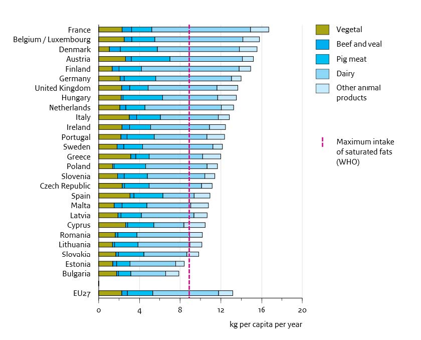
| [113] | Henk Westhoek et al. (2011) The protein puzzle, the consumption and production of meat, dairy and fish in the European Union. Netherlands Environmental Assessment Agency. [online] |
| [114] | European Commission (2012) Consultation paper: options for resource efficiency indicators. [online] |
| [115] | International Agency for Research on Cancer (2015) Press release. IARC Monographs evaluate consumption of red meat and processed meat. online. Red meat includes beef, pork, lamb and mutton, goat |
| [116] | World Cancer Research Fund. Red and processed meat and cancer prevention. online. Referring to meats which are preserved through smoking, curing, salting or through addition of preservatives, including ham, salami, bacon, sausages, hot dogs etc. |
| [117] | World Cancer Research Fund, American Institute of Cancer Research (2007) Second Expert Report: Food, Nutrition, Physical activity and the Prevention of Cancer: a Global Perspective. [online] |
| [118] | Henk Westhoek et.al. (2014) Food choices, health and environment: Effects of cutting Europe's meat and dairy intake. Global Environmental Change. [online] |
| [119] | Mark Sutton et al. (ed) (2011) The European Nitrogen Assessment. Sources, effects and policy perspectives. [online] |
| [120] | European Commission (2004) The meat sector in the European Union. [online] |
| [121] | See for instance: World Resource Institute. Data series: Meat consumption per capita. [online] |
| [122] | European Commission (1980) Agriculture and the problem of surpluses. p. 18-19. [online] |
| [123] | Article 52 Direct payments Regulation |
| [124] | Article 53 Direct payments Regulation |
| [125] | 15% from all net ceilings added up. See Annex III Direct payments Regulation. |
| [126] | European Commission. EU Draft Budget for 2016. online. Budget lines starting from code 05. |
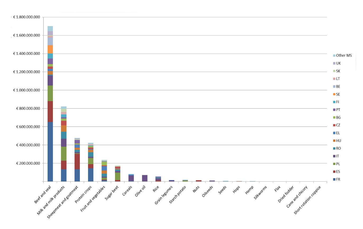
| [127] | Alan Mathews (2015) Two steps forward, one step back: coupled payments in the CAP. CAPreform.eu. [online] |
| [128] | European Commission (2014) The CAP towards 2020. Implementation of the new system of direct payments. MS notifications. [online]. Promoting protein crop production in Europe can however be considered positive as a way to replace soy import from South America. |
| [129] | European Court of Auditors (2012) Suckler cow and ewe and goat direct aids under partial implementation of SPS arrangements. online. Both these schemes expired in 2014 together with Regulation (EC) No 73/2009 on direct support schemes for farmers under the common agricultural policy. |
| [130] | Article 52(8) Direct payment Regulation |
| [131] | Article 26 CMO Regulation and further |
| [132] | European Parliament Procedure File 2014/0014 COD. Aid scheme for the supply of fruit and vegetables, bananas and milk in the educational establishments. online. See also: Text adopted in EP Plenary on 27 May. [online] |
| [133] | Eurostat (2011) Food: From farm to fork statistics. [online] |
| [134] | FAO. Milk and Dairy products in human nutrition - questions and answers. [online] |
| [135] | FAO. Food-based dietary guidelines, Food guidelines by country. online. . For criticism on reduced fat milk see for instance: David Ludwig et al. (2011) Three daily servings of reduced-fat milk - an evidence based recommendation? JAMA Pediatrics. [online] |
| [136] | Articles 11 and 16 CMO Regulation |
| [137] | Article 17 CMO Regulation |
| [138] | European Commission (2015) Private storage in the pig meat sector. [online] |
| [139] | European Commission Press release (2015) Safety net measures for dairy, fruit and vegetables to be extended. [online] |
| [140] | Article 196 CMO Regulation |
| [141] | Article 219 CMO Regulation. See also: Alan Mathews (2013) The end of export subsidies? CAPreform.eu. [online] |
| [142] | Article 220 CMO Regulation |
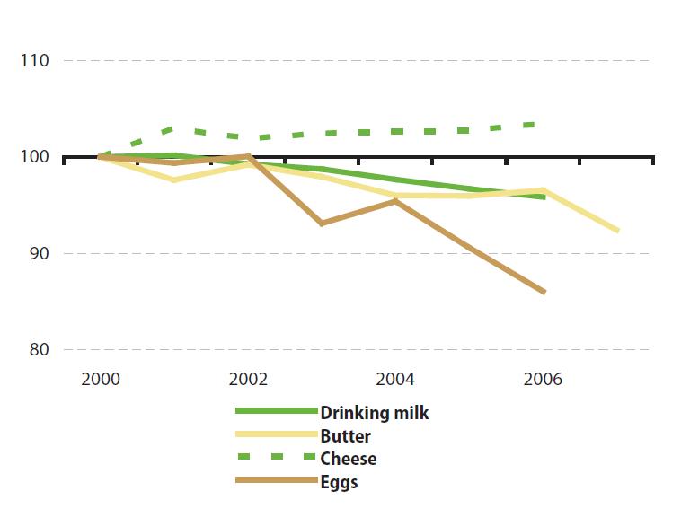
| [143] | European Parliament Resolution of 7 July 2015 on prospects for the EU dairy sector - review of the implementation of the Dairy Package online. See also: European Parliament News (2015) End of milk quotas: “Opportunities to build a more confident and robust dairy sector”. [online] |
| [144] | Euractiv (2014) Moscow pork embargo causes havoc in Brussels. [online] |
| [145] | AHDB Dairy (2015) EU Farmgate milk prices. [online] |
| [146] | Copa-Cogeca Press release (2015) Copa and Cogeca warn at EU Milk Market Observatory meeting market deteriorated rapidly in past 4 weeks and EU action crucial. online. See also: Euractiv (2015) France promises emergency aid to farmers, online. & Euractiv (2015), Farmers look to EU food aid to boost meat market. [online] |
| [147] | See for instance: VILT.be (2015) Landbouworganisaties komen met gemeeschappelijke eisen. online. A coalition of Belgian farmers' organizations demands what farmers really want i.e. fair prices. |
| [148] | Aileen Robertson et al. (ed) (2004) Food and health in Europe: a new basis for action. WHO Europe. [online] |
| [149] | M. Crawford et al. (1970) Comparative studies on fatty acid composition of wild and domestic meats. International Journal of Biochemistry. [online] |
| [150] | Compassion in World Farming (2012) Nutritional benefits of higher welfare animal products. [online] |
| [151] | B. H. Schwendel et al. (2014) Organic and conventionally produced milk - An evaluation of factors influencing milk quality. Journal of Dairy Science. [online] |
| [152] | Liesbet Smit et al. (2010) Conjugated linoleic acid in adipose tissue and risk of myocardial infarction. The American Journal of Clinical Nutrition. [online] |
| [153] | Compassion in World Farming, World Society for the Protection of Animals (2013) Zoonotic diseases, human health and farm animal welfare. [online] |
| [154] | WHO (2015) Healthy Diet. Fact sheet No 394. [online] |
| [155] | EUFIC (2012) Fruit and vegetables consumption in Europe - do Europeans get enough? [online] |
| [156] | European Association for the Fresh Fruit and Vegetables Sector (2015) Freshfel Consumption Monitor. [online] |
| [157] | AFC Management Consulting (2012) Evaluation of the European School Fruit Scheme - Final report. For the European Commission. [online] |
| [158] | WHO (2009) Global Health Risks Summary Tables. [online] |
| [159] | Article 23 CMO Regulation and further |
| [160] | European Parliament Procedure File 2014/0014 COD. Aid scheme for the supply of fruit and vegetables, bananas and milk in the educational establishments. online. See also: Text adopted in EP Plenary on 27 May. [online] |
| [161] | See for instance: Joint Open letter: Save the EU School Fruit Scheme: ‘Better Regulation' cannot go against the wellbeing of European children (2015). [online] |
| [162] | European Court of Auditors (2011) Are the School milk and School fruit schemes effective? [online] |
| [163] | AFC Management Consulting (2012) Evaluation of the European School Fruit Scheme - Final report. For the European Commission. [online] |
| [164] | Processed fruits and vegetables are allowed but without added sugar, added fat, added salt, added sweeteners and/or artificial flavour enhancers (artificial food additive codes E620-E650) |
| [165] | European Parliament Policy Study (2011) The EU Fruit and vegetables sector: overview and post-2013 CAP perspective. [online] |
| [166] | Article 32 CMO Regulation and further |
| [167] | European Commission. EU Draft Budget for 2016. online. Budget lines starting with code 05. |
| [168] | European Parliament Policy Study (2015) Towards new rules for the EU's fruit and vegetables sector. [online] |
| [169] | Schäfer Elinder (2003) Public health aspects of the EU Common Agricultural Policy. Developments and recommendations for change in four sectors: Fruit and vegetables, dairy, wine and tobacco. National Institute of Public Health, Sweden |
| [170] | Lennert Veerman et al. (2005) The European Common Agricultural Policy on fruits and vegetables: exploring potential health gain from reform. European Journal of Public Health. [online] |
| [171] | European Commission. Fruit and vegetables: crisis prevention and management. [online] |
| [172] | Steve Wiggins et al. (2015) The rising cost of a healthy diet - changing relative prices of food in high income and emerging economies. Overseas Development Institute, UK. [online] |
| [173] | European Parliament resolution of 7 July 2015 on the fruit and vegetables sector since the 2007 reform. [online] |
| [174] | Luciano Trentini (2015) Les fruits et légumes européens dans le monde. Fruit and Horticultural European Regions Assembly. [online] |
| [175] | Luciano Trentini (2015) Fruit and Horticultural European Regions Assembly. [online] |
| [176] | Jos Bijman (2015) Towards new rules for the EU's fruit and vegetables sector. European Parliament policy study. [online] |
| [177] | European Heart Network (2008) Response to “Towards a possible European school fruit scheme - Consultation document for impact assessment”. [online] |
| [178] | Karen Lock et al. (2005) Fruit and vegetable policy in the European Union: Its effects on the burden of cardiovascular disease. London School of Hygiene and Tropical Medicine, European Heart Network. [online] |
| [179] | European Parliament resolution of 7 July 2015 on the fruit and vegetables sector since the 2007 reform. [online] |
| [180] | An Ruopeng (2015) Nationwide Expansion of a Financial Incentive Program on Fruit and Vegetable Purchases among Supplemental Nutrition Assistance Program Participants: A Cost-effectiveness Analysis. Social Science & Medicine. [online] |
| [181] | F. Ford et al. (2009) Effect of the introduction of ‘Healthy start' on dietary behaviour during and after pregnancy: early results from the ‘before and after'. [online] |
| [182] | European Commission (2014) First Commission interim report on the implementation of Pilot Projects and Preparatory Actions 2014. [online] |
| [183] | Anne-Marie Mayer (1997) Historical changes in the mineral content of fruits and vegetables. British Food Journal. [online] |
| [184] | Aileen Robertson et al. (ed) (2004) Food and health in Europe: a new basis for action. WHO Europe. [online] |
| [185] | See: Directive 2009/128/EC establishing a framework for Community action to achieve the sustainable use of pesticides. [online] |
| [186] | European Commission (2015) Annex Promotion on the internal market and in third countries. online. See also: European Commission Press release (2015) The Commission approves new promotion programmes for agricultural products. [online] |
| [187] | European Commission (2014) Formal adoption of new EU promotion rules for agricultural products. [online] |
| [188] | European Commission (2015) The new promotion policy. Synoptic presentation. [online] |
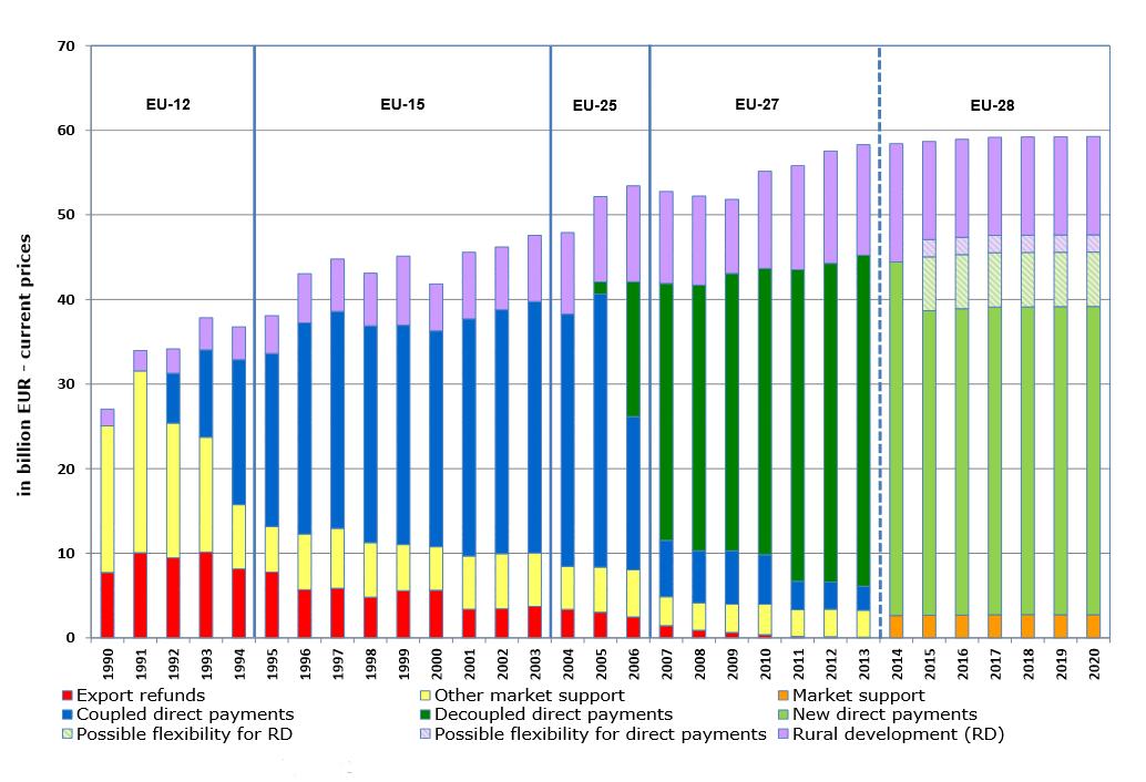
| [189] | Regulation (EU) No 1144/2014 on information provision and promotion measures. [online] |
| [190] | Graph: European Commission (2013) Overview of CAP Reform 2014-2020. online. First pillar funding amount is in current prices. |
| [191] | European Commission DG AGRI (2011) The Future of CAP Direct Payments. [online] |
| [192] | Article 25 and further Direct Payments Regulation |
| [193] | European Parliament Policy Study (2015) Implementation of the First Pillar of the CAP 2014-2020 in the EU Member States. [online] |
| [194] | European Commission DG AGRI (2013) CAP reform - an explanation of the main elements. [online] |
| [195] | Article 36 Direct Payments Regulation |
| [196] | Article 21 Direct Payments Regulation |
| [197] | See for instance: Alan Mathews (2009) How decoupled is the single farm payment? CAPreform.eu. [online] |
| [198] | The Economist (2005) Europe's farm follies. [online] |
| [199] | European Parliament Policy Study (2015) Extent of Land Grabbing in the EU. [online] |
| [200] | Article 41 and further Direct payments Regulation |
| [201] | Article 61 and further Direct payments Regulation |
| [202] | Article 11 Direct payments Regulation |
| [203] | European Commission DG AGRI (2013) Structure and dynamics of EU farms: changes, trends and policy relevance. [online] |
| [204] | European Commission (2010) Does population decline lead to economic decline in EU rural regions? [online] |
| [205] | The Economist (2015) Rural France. Village croissant. [online] |
| [206] | WHO Europe (2012) Addressing the social determinants of health: the urban dimension and the role of local government [online] |
| [207] | John Bryden et al. (2004) Rural development and food policy in Europe. In: London School of Economics and Political Science. Eurohealth issue: Integrating Public Health with European food and agricultural policy. [online] |
| [208] | European Parliament Policy Study (2015) Towards new rules for the EU's fruit and vegetables sector. [online] |
| [209] | Article 5 Direct payments Regulation referring to Regulation (EU) online. which contains the list of cross-compliance measures in Annex II |
| [210] | European Council of the European Union. Simplification of the EU's Common Agricultural Policy (CAP). [online] |
| [211] | Article 43 and further Direct payments Regulation |
| [212] | Directive 2009/128/EC establishing a framework for Community action to achieve the sustainable use of pesticides |
| [213] | Recital 2 Rural development Regulation |
| [214] | European Commission (2013) Overview of CAP Reform 2014-2020. [online]. In current prices. Rural development measures, unlike direct payments or market measures, are co-financed by Member States. |
| [215] | Article 13 and further Rural development Regulation |
| [216] | Joris Aertsen et.al. (2013) Valuing the carbon sequestration potential for European agriculture. Land Use Policy. [online] |
| [217] | FAO (2013) Advancing agroforestry on the policy agenda. [online] |
| [218] | European Commission (2014) Investment support under Rural Development Policy. online. Implementation of the First Pillar of the CAP 2014-2020 in the EU Member States |
| [219] | European Court of Auditors (2014) Special report no 23/2014: Errors in rural development spending: what are the causes, and how are they being addressed? [online] |
| [220] | Article 14 Direct payments Regulation. See also: Wageningen University, IEEP (2009) Study on the impact of modulation. [online] |
| [221] | European Parliament Policy Study (2015) Implementation of the First Pillar of the CAP 2014-2020 in the EU Member States. [online] |
| [222] | FAO (2012) Sustainable diets and biodiversity. Directions and solutions for policy research and action. Proceedings of International Scientific Symposium. [online] |
| [223] | European Commission (2011) Evaluation of effects of direct support on farmers' incomes. [online] |
| [224] | Eurostat. Cross-country comparison of final consumption expenditures on food and housing in 2011. online. In UK and Luxembour the average is below 10%, while in Latvia and Estonia it is near 20% of total expenditure. |
| [225] | OECD (2012) Income inequality in the European Union. [online] |
| [226] | UCL Institute of Health Equity (2014) Review of social determinants and the health divide in the WHO European Region: final report. WHO Europe. [online] |
| [227] | Eurostat data in: Euractiv (2014) One out of four EU citizens at risk of poverty. [online] |
| [228] | Aileen Robertson et al. (2007) Obesity and socio-economic groups in Europe: Evidence review and implications for action. Report for European Commission. [online] |
| [229] | A. Drewnowski (2009) Obesity, diets and social inequality, Nutrition Reviews, online. See also: WHO (2012) Environmental Health Inequalities in Europe. [online] |
| [230] | Belinda Loring et al. (2014) Obesity and inequities Guidance for addressing inequities in overweight and obesity. [online] |
| [231] | European Commission (2005) The contribution of health to the economy in the European Union. [online] |
| [232] | Lancet Commission on planetary health (2015) Safeguarding human health in the Anthropocene epoch. The Lancet. [online] |
Figures(10)

Nikolai Pushkarev. A CAP for Healthy LivingMainstreaming Health into the EU Common Agricultural Policy


 DownLoad: