
Citation: Sujit Nair. Current insights into the molecular systems pharmacology of lncRNA-miRNA regulatory interactions and implications in cancer translational medicine[J]. AIMS Molecular Science, 2016, 3(2): 104-124. doi: 10.3934/molsci.2016.2.104
[1] | K. Wayne Forsythe, Cameron Hare, Amy J. Buckland, Richard R. Shaker, Joseph M. Aversa, Stephen J. Swales, Michael W. MacDonald . Assessing fine particulate matter concentrations and trends in southern Ontario, Canada, 2003–2012. AIMS Environmental Science, 2018, 5(1): 35-46. doi: 10.3934/environsci.2018.1.35 |
[2] | Carolyn Payus, Siti Irbah Anuar, Fuei Pien Chee, Muhammad Izzuddin Rumaling, Agoes Soegianto . 2019 Southeast Asia Transboundary Haze and its Influence on Particulate Matter Variations: A Case Study in Kota Kinabalu, Sabah. AIMS Environmental Science, 2023, 10(4): 547-558. doi: 10.3934/environsci.2023031 |
[3] | Anna Mainka, Barbara Kozielska . Assessment of the BTEX concentrations and health risk in urban nursery schools in Gliwice, Poland. AIMS Environmental Science, 2016, 3(4): 858-870. doi: 10.3934/environsci.2016.4.858 |
[4] | Nikolaos Barmparesos, Vasiliki D. Assimakopoulos, Margarita Niki Assimakopoulos, Evangelia Tsairidi . Particulate matter levels and comfort conditions in the trains and platforms of the Athens underground metro. AIMS Environmental Science, 2016, 3(2): 199-219. doi: 10.3934/environsci.2016.2.199 |
[5] | Novi Sylvia, Husni Husin, Abrar Muslim, Yunardi, Aden Syahrullah, Hary Purnomo, Rozanna Dewi, Yazid Bindar . Design and performance of a cyclone separator integrated with a bottom ash bed for the removal of fine particulate matter in a palm oil mill: A simulation study. AIMS Environmental Science, 2023, 10(3): 341-355. doi: 10.3934/environsci.2023020 |
[6] | Dimitrios Kotzias . Built environment and indoor air quality: The case of volatile organic compounds. AIMS Environmental Science, 2021, 8(2): 135-147. doi: 10.3934/environsci.2021010 |
[7] | Winai Meesang, Erawan Baothong, Aphichat Srichat, Sawai Mattapha, Wiwat Kaensa, Pathomsorn Juthakanok, Wipaporn Kitisriworaphan, Kanda Saosoong . Effectiveness of the genus Riccia (Marchantiophyta: Ricciaceae) as a biofilter for particulate matter adsorption from air pollution. AIMS Environmental Science, 2023, 10(1): 157-177. doi: 10.3934/environsci.2023009 |
[8] | Andrea L. Clements, Matthew P. Fraser, Pierre Herckes, Paul A. Solomon . Chemical mass balance source apportionment of fine and PM10 in the Desert Southwest, USA. AIMS Environmental Science, 2016, 3(1): 115-132. doi: 10.3934/environsci.2016.1.115 |
[9] | Cristina Calderón-Tapia, Edinson Medina-Barrera, Nelson Chuquin-Vasco, Jorge Vasco-Vasco, Juan Chuquin-Vasco, Sebastian Guerrero-Luzuriaga . Exploration of bacterial strains with bioremediation potential for mercury and cyanide from mine tailings in "San Carlos de las Minas, Ecuador". AIMS Environmental Science, 2024, 11(3): 381-400. doi: 10.3934/environsci.2024019 |
[10] | Barend L. Van Drooge, David Ramos García, Silvia Lacorte . Analysis of organophosphorus flame retardants in submicron atmospheric particulate matter (PM1). AIMS Environmental Science, 2018, 5(4): 294-304. doi: 10.3934/environsci.2018.4.294 |
The keys for quantitative analysis of plant traits are accurate and efficient collection of genetic and phenotypic data. Compared to recent advances in large-scale genetic information collection, the classical hand-measured approach for collecting plant traits is labor-intensive and inefficient. High-throughput image-based phenotyping systems have recently been built to overcome this problem. Substantial advancements have been made by engineers to enable the large-scale collection of plant images and sensor data [1,2,3,4,5]. A unifying objective among researchers is the accurate extraction of plant traits from images [6,7]. While systems able to produce thousands of images per day exist, the raw images are often only stepping stones to further analysis. For this reason, an important current area of research involves obtaining plant traits from raw images that can then be used in downstream analyses. A host of image analysis techniques from the field of computer vision are often applied to extract various plant traits, and, increasingly, machine learning algorithms are being applied to improve the accuracy of the measurements as well as the efficiency and scalability of the process [8,9,10,11,12].
A common approach to extracting a number of plant measurements from images first requires binary images to be produced through the process of image segmentation. Methods such as frame differencing [13], K-means [14,15], and thresholding [16,17] are frequently used. In [18], a neural network model was trained to classify each pixel in a maize image into either the plant class or the background class. It was demonstrated that the neural network segmentation is more accurate and robust than the traditional methods mentioned above. However, such a segmentation method based on a neural network is time consuming for high resolution images and the high-throughput phenotyping systems that produce large numbers of plant images daily for experiments.
In recent years, convolutional neural networks have become a standard approach for many image analysis tasks (see, for instance, [19,20,21,22,23]). They have achieved state-of-the-art results in a number of challenging areas. The main advantage of CNNs over standard feed-foward neural networks for image analysis is, by means of convolutional layers, CNNs can preserve local structural information. Intuitively, pixels are not scattered independently throughout an image. In the case of plant images, plant pixels are more likely to be next to or surrounded by other plant pixels while background pixels are more likely to be surrounded by other background pixels. Because of the preservation of local information, CNNs are thus able to learn to recognize quite complicated features with far fewer parameters than would be required of a feed-forward network [24,25].
There have been an increasing number of applications of deep neural networks to plant phenotype extraction from images in recent years. Miao, et al. [26] employed a relatively shallow convolutional neural network (CNN) for leaf counting of maize plants. Trained using a combination of real maize images from a greenhouse and simulated maize images, this network learned to accurately count maize leaves. Lu, et al. [27] used deeper CNN structures to count the number of tassels on maize plants in an unconstrained field environment. Using 186 images for training and validation, several CNN structures were adapted from well-known models and retrained to enable accurate tassel counts. A multi-task CNN was trained in [28] to simultaneously identify wheat images containing spikes and spikelets as well as to localize and thus count said spikes and spikelets. Their CNN architecture makes use of residual blocks [29] and skip-training [30] to achieve near-perfect accuracy in spike and spikelet counting. Aich, et al. [31] utilized CNNs for estimating emergence and biomass of wheat plants from high-resolution aerial field images. The SegNet [32] architecture was used for soft segmentation as part of extracting both emergence and biomass, and a CNN utilizing inception blocks [33] and inception-residual blocks [34] was trained for each of their desired traits. In those works, CNNs with millions of parameters were constructed and estimated on limited training data. However, such large networks trained on a small amount of data may not be stable or accurate for trait prediction.
As a well-trained CNN requires a large amount of training data which may not be available in many applications, transfer learning [35] borrows the structures of pre-trained networks to solve this problem. In transfer learning, parts of a previously trained CNN are incorporated into a new network. This allows portions of a model trained for a specific task, say object classification, to be used in a different model for a different task, say object localization. A number of the most well-known and top-performing models for many image analysis tasks have been made publicly available [19,20,36]. Thus not only does transfer learning reduce the need for extensive computational resources, it can also apply portions of the best CNNs to new tasks. Both the computational efficiency and improvement in task performance resulting from transfer learning have been demonstrated in a number of cases across various research domains [37,38,39,40].
This paper considers the implementation of CNNs with transfer learning to directly predict plant trait measurements from greenhouse images without segmentation. The images considered here are RGB images of soybean plants taken at the University of Nebraska-Lincoln Greenhouse Innovation Center; see Figure 1 for examples of soybean plant images. As preparing training data with accurate measurements for plant traits is both labor and time consuming, in this paper, we apply the idea of transfer learning based on the model known as VGG16 [19], which is a deep CNN originally trained for image classification on the ImageNet data set [41]. By borrowing the network structure and its parameters from the pre-trained model, we reduce the number of parameters that must be estimated in our model.
Table 1 describes the architecture of the original VGG16 model, which used $ 224 \times 224 $ pixel RGB images as input. We pass all the soybean images to the VGG16 network and obtain the flattened vector of output from its 18th layer in Table 1. Those vectors of output are then treated as the input layer for a fully connected neural network for predicting the soybean traits. The proposed approach can be viewed as a neural network prediction method applied on the transferred images by the VGG16 model. Note that the layers 19–21 in VGG16 are not implemented in our model. More details on the implementation of the proposed method are given in the Materials and Methods section.
Layer Number | Layer Type | Details |
1 | Convolutional Layer | 64 filters of size $3 \times 3 \times 3$, stride of 1, ReLU activation |
2 | Convolutional Layer | 64 filters of size $3 \times 3 \times 64$, stride of 1, ReLU activation |
3 | Max Pooling Layer | $2 \times 2$ kernel, stride of 2 |
4 | Convolutional Layer | 128 filters of size $3 \times 3 \times 64$, stride of 1, ReLU activation |
5 | Convolutional Layer | 128 filters of size $3 \times 3 \times 128$, stride of 1, ReLU activation |
6 | Max Pooling Layer | $2 \times 2$ kernel, stride of 2 |
7 | Convolutional Layer | 256 filters of size $3 \times 3 \times 128$, stride of 1, ReLU activation |
8 | Convolutional Layer | 256 filters of size $3 \times 3 \times 256$, stride of 1, ReLU activation |
9 | Convolutional Layer | 256 filters of size $3 \times 3 \times 256$, stride of 1, ReLU activation |
10 | Max Pooling Layer | $2 \times 2$ kernel, stride of 2 |
11 | Convolutional Layer | 512 filters of size $3 \times 3 \times 256$, stride of 1, ReLU activation |
12 | Convolutional Layer | 512 filters of size $3 \times 3 \times 512$, stride of 1, ReLU activation |
13 | Convolutional Layer | 512 filters of size $3 \times 3 \times 512$, stride of 1, ReLU activation |
14 | Max Pooling Layer | $2 \times 2$ kernel, stride of 2 |
15 | Convolutional Layer | 512 filters of size $3 \times 3 \times 512$, stride of 1, ReLU activation |
16 | Convolutional Layer | 512 filters of size $3 \times 3 \times 512$, stride of 1, ReLU activation |
17 | Convolutional Layer | 512 filters of size $3 \times 3 \times 512$, stride of 1, ReLU activation |
18 | Max Pooling Layer | $2 \times 2$ kernel, stride of 2 |
Flattening | Flatten array resulting from layer 18 into 1-D vector | |
19 | Fully-connected Layer | 4096 units, ReLU activation, Dropout with dropout probability 0.5 |
20 | Fully-connected Layer | 4096 units, ReLU activation, Dropout with dropout probability 0.5 |
21 | Fully-connected Layer | Output layer, 1000 units, Softmax activation |
It will be demonstrated that our approach using less than 2000 training images can accurately produce plant trait measurements from greenhouse RGB images of soybean plants. Using available hand-measured height data, we will also demonstrate the superiority of CNN height prediction to the heights obtained from the method based on image segmentation. Those results indicate our transfer learning approach successfully implements a large neural networks trained on a relatively small sets of plant images. This advantage could be important to save time and labor in many plant phenotyping research, as different training data need to be separately prepared for different plants and experiments. With this use of transfer learning on greenhouse soybean images, our CNN method constitutes a novel approach to trait extraction from high-throughput phenotyping systems.
In this study, the only hand-measurement we are able to access is the soybean plant height as measured in inches. However, the main purpose of this paper is to demonstrate the utility of machine learning to extract various trait measurements from these plant images. As such, we demonstrate the ability of CNNs to accurately predict the height, width, and what we will refer to as the size of a plant as obtained from the binary segmented images of soybean plants. These thus stand in as proxies for actual trait measurements which a CNN could be trained to obtain given hand-measured trait data. A description of how these measurements are obtained through image segmentation is given in section 2.2. We also use the hand-measured height data to train a CNN solely for height prediction to show that CNNs can be both more accurate and more efficient than the image segmentation-based method.
In summary, this paper presents two related novel contributions. First, we make use of transfer learning in training a CNN to directly extract phenotypic traits from soybean plants. That is, with no image preprocessing other than resizing, our model takes raw RGB images and predicts the plant traits on a standard measurement scale. Using this approach, we have outperformed previous state-of-the-art results in the tasks considered. Second, by incorporating part of the VGG16 model into the first layers of our model, we have been able to achieve our superior performance more efficiently relative to other, similar work in image analysis. That is, we required relatively small amount of training images and used less computation time to obtain our results. Thus this paper contributes to the field of plant phenomics by providing an efficient and accurate means of plant trait extraction via deep learning methods.
There are a total of 15,223 sets of images of soybean plants in this experiment, taken from January to May 2018. Each image has a resolution of $ 2056 \times 2454 $ pixels. There is also a subset of 2235 images for which hand-measured heights are available. The high-throughput imaging system also records millimeter-per-pixel information for each image taken that allows for converting estimated trait measurements from pixel scale to standard scales (e.g., inches in the case of height).
Of the total available image sets, two separate collections of image data were created for trait extraction. The first collection consists of 2000 images sampled at random from the total 15,223 images. As hand-measured heights were not available for all of these images, the height, width, and size measurements were obtained through segmentation (see the following subsection). This image collection will be referred to as the segmentation-obtained, or SO, collection. To predict the plant traits by CNN, this collection was split into training and testing sets. The SO training set consists of 1800 images while the SO testing set consists of the remaining 200 images from the SO collection.
The second image collection contains all 2235 images for which hand-measured heights are available. As such, this collection will be referred to as the hand-measured, or HM, collection. Similar to the SO collection, the HM collection was split into training and testing sets. The HM training set contains 1938 images while the HM testing set contains the remaining 297 images.
All images in both collections were scaled down from their original size of $ 2056 \times 2454 $ pixels to $ 1024 \times 1227 $ pixels by the resize function from the OpenCV Python library. This was done to reduce the amount of computation time needed for the methods employed.
To obtain the height, width, and size measurements of plants via segmentation, the method of obtaining training data for image segmentation by a combination of cropping and K-means as described in [18] was employed. This process yielded a data set containing 9,325,817 total pixels as observational units. Of these, 8,857,179 were labeled as background pixels and 468,368 were plant pixels. A neural network with the same architecture as was employed for maize segmentation in [18] was then trained on these data. Once the segmentation model was trained, all images in the SO collection were segmented to binary images with 1 and 0 standing for plant and background pixels respectively. To further reduce the background noise for better trait measurements, each binary image was subjected to a morphological opening which employed the $ 5 \times 5 $ diamond-shaped kernel matrix [42,43]. This was accomplished using the morphologyEx function from the OpenCV Python library. The desired plant trait measurements could then be obtained from those segmented images. Furthermore, the HM testing set images were also segmented. This was done to allow for comparison of the segmented heights with the hand-measured heights. The Keras library in Python was used for training and prediction of the segmentation model.
As the hand-measured height was taken from the top of the pot to the top of the plant, the segmentation-obtained height in terms of pixels was calculated by taking the difference between the top of the pot and the uppermost $ y $-position of the plant in the image. Note that the location of the pot is uniformly the same in all images under consideration. Similarly, the difference between the right-most and the left-most $ x $-positions of a plant yields the pixel width of the plant. The millimeter-per-pixel information of the images, which is available for both the $ x $ and $ y $ directions, were then used to scale the height and width to inches. Finally the size of the plant was obtained by simply summing the total number of plant pixels in each binary image. Again using millimeter-per-pixel information, the measurement was then scaled to square inches.
All three traits under consideration serve a practical purpose. The different experimental lines and exotic germplasm used in this study express their phenotypes along a spectrum of variation for a given trait. In this experiment, we used a set of soybean germplasm rich in genetic diversity and thus, in phenotypic variation. Of the traits under consideration, height is often used to reveal the plant growth dynamic, and its association with genetic variation. In addition to growth dynamic, plant biologists are also interested in plant architecture. In this scenario, plant width refers specifically to above-ground plant horizontal architecture. This is related to differences in petiole length, branch length, branch size, leaf length, overall plant size, among others. Similarly, plant size as measured by the millimeter-per-pixel information of the images, is a proxy for above-ground plant biomass. Hand-measurements of plant width (horizontal architecture) and size (a destructive measurement of above-ground biomass) would not only be cumbersome, but also very difficult to obtain. Therefore, the two-dimensional information provided by these measurements is significant for characterization of plant architecture.
The Keras library in Python was used for training and prediction of the convolutional neural network. In order to predict the height, width, and size from the SO images as well as the height from the HM image collection, four separate networks were trained. These are referred to, respectively, as CNN-HSO, CNN-WSO, CNN-SSO, and CNN-HHM. While the four models learn different parameters during the training process, they all utilize the same network architecture.
As mentioned in the introduction, layers, including the pre-trained parameters, from the VGG16 model were implemented as part of our network architecture. Specifically, layers 1–18 from Table 1 served as the layers of our CNN architecture. The output from the 18th layer of the VGG16 portion of our CNN architecture was a $ 32 \times 38 \times 512 $ array. This array was then flattened into a column vector of 622,592 units which was then fed into a fully-connected neural network with 2 hidden layers of 64 units, both of which use the ReLU activation function [25,44]. Finally, the output layer consists of only one unit and employs the linear activation function. As the plant traits are non-negative, the negative predicted values from the proposed models were replaced by 0. This fully connected portion of our neural network architecture contains 39,850,177 parameters that need to be trained for each of the four CNNs.
In addition to having the same architecture, all four CNNs were trained using the same choices of loss function, optimizer, etc. The loss function was the mean squared error, and the Adam optimizer was used with learning rate $ \alpha = 0.0008 $ and recommended exponential decay rates of $ \beta_1 = 0.9 $ and $ \beta_2 = 0.999 $ [44,45]. The models were each trained in batches of 128 images and ran for 100 epochs [25]. The CNN-HSO, CNN-WSO, and CNN-SSO networks were trained on the 1800 images in the SO training set and evaluated on the 200 images in the SO testing set. The CNN-HHM network was trained on the 1938 images in the HM training set and evaluated on the 297 images in the HM testing set. Note that the hyperparameters were tuned by randomly holding out 10% of the training observations as validation data and finding values that minimized the loss on the validation set of images. Once the hyperparameters were selected, the models were retrained on the entire training data sets.
As computational time is an important consideration in image analysis tasks, the time needed to extract plant trait measurements from a $ 1028 \times 1227 $ pixel image was measured for all four CNNs as well as for the height extraction based on segmentation. To accomplish this, one image was selected at random from the SO image collection. This image served as the input for 100 runs of each of the four CNNs. There were also 100 runs where a binary image was produced by the segmentation model and the height was calculated as described in section 2.2. Note that only the time for height extraction was calculated from the segmentation-based method as the computation time required for any of the height, width, and size measurements from segmented images is negligible.
Panels (a) and (b) of Figure 2 show an RGB soybean image and the corresponding binary image resulting from the proposed segmentation method. From visual inspection, our method appears to produce a well-segmented binary image. Panel (c) of Figure 2 contains the heights obtained from the binary images in the HM test set plotted against the hand-measured heights from those same images. The closer a point is to the 45 degree line seen in the plot, the smaller the discrepancy between hand-measured height and segmentation-obtained height for a given image. The mean absolute deviation between hand-measured and segmentation-obtained heights for the HM test set is 0.83. That is, for these images, the average discpreancy between measured and predicted height is only 0.83 inches. This demonstrates that our image segmentation-based approach to height extraction is viable.
We first consider the results of the CNN-HSO, CNN-SSO, and CNN-WSO models. Figure 3(b)–(d) contain, for each of these three models, the predicted traits plotted against the traits extracted from the binary versions of the SO testing set images. Each of these plots contains a black 45 degree line representing where the predicted and observed traits are equal. In panels (b) and (c), the blue dotted lines represent deviations of 1 inch between predicted and observed heights and widths, respectively. Similarly, the red dotted lines represent deviations of 2 inches for those traits. For the size plot in panel (d), the blue dotted lines represent a deviation of 1 square inch while the red dotted lines represent a deviation of 4 square inches.
Some basic measures to assess the quality of the predictions are found in Table 2. These are the mean absolute deviation, the $ R^2 $, and the proportions of absolute deviations falling into given regions. For the CNN-HSO and CNN-WSO, region one is less than 1 inch, region two is at least 1 inch but less than two inches, region three is at least 2 inches but less than 3 inches, and region four is at least 3 inches. As CNN-SSO predicts size, which is measured here in square inches, the regions change so that region one contains deviations less than 1 square inch, region two is at least 1 square inch but less than 4 square inches, region three is at least 4 square inches but less than 9 square inches, and region four is at least 9 square inches.
CNN-HSO | CNN-WSO | CNN-SSO | |
MAD | 1.11 in. | 0.8633 in. | 1.51 sq in. |
$R^2$ | 0.9707 | 0.9444 | 0.9723 |
Prop. Region 1 | 0.610 | 0.665 | 0.565 |
Prop. Region 2 | 0.225 | 0.250 | 0.345 |
Prop. Region 3 | 0.080 | 0.050 | 0.075 |
Prop. Region 4 | 0.085 | 0.035 | 0.015 |
From Table 2, the average deviations between predicted and segmentation-obtained traits are small and the $ R^2 $ values are close to 1. Further, for each model, more than 83% of all deviations fall in regions 1 and 2. For CNN-WSO and CNN-SSO, over 91% of the deviations are in regions 1 and 2. Thus, from each model, only a small proportion of the total images result in egregious deviations. Possible reasons for these deviations will be explored in the Discussion section. Overall, these measures indicate that all three models are capable of extracting the desired trait measurements accurately.
The CNN-HHM model was trained and evaluated on the HM image collection (using the HM training and testing sets, respectively). Panel (a) of Figure 3 shows that the CNN-HHM predicted heights are quite close to the hand-measured heights on the testing data set. The lines in the plot correspond to those seen in panels (b) and (c) of Figure 3. Recall that Panel (c) in Figure 2 plots the height obtained from segmentation against the hand-measured heights for all 297 HM testing images. We compare the accuracy of CNN-HHM prediction to the method based on segmentation.
Table 3 contains the same measurements as those given in Table 2 for the segmentation-obtained and CNN-HHM predicted heights on the 297 HM testing set images. The regions for Table 3 are the same as those used for CNN-HSO and CNN-WSO. Here we notice that, on average, the CNN-HHM predicted heights are just over half of an inch from the hand-measured heights. This is a big improvement over the segmentation-obtained heights, whose mean absolute deviation is 0.8348 (which is still a good result). The $ R^2 $ values are comparable between the two methods with the segmentation-obtained $ R^2 $ just a little larger. The CNN-HHM also outperforms the segmentation heights in terms of the proportion of deviations within an inch of the hand-measured height. Just over 90% of CNN-HHM predictions lie within an inch of the actual height while the value is close to 73% for the segmentation-obtained heights. The one area in which the segmentation-obtained heights appear to do better than the CNN-HHM predicted heights can be observed from the plot in Figure 3(a). It appears that even though most of the deviations in this plot are smaller than the deviations in panel (c) of Figure 2 (i.e., they are more tightly clustered around the 45 degree line), there are some exceptionally large deviations produced by the CNN-HHM predictions. As with the other three CNN models, only a small percentage of images produce egregious deviations from the hand-measured heights. These will also be investigated further in the Discussion section. Overall, it appears that CNN-HHM extracts the soybean height more accurately than the segmentation method does.
Segmentation-obtained | CNN-HHM | |
MAD | 0.8348 in. | 0.5236 in. |
$R^2$ | 0.9758 | 0.9698 |
Prop. Region 1 | 0.7273 | 0.9057 |
Prop. Region 2 | 0.2290 | 0.0606 |
Prop. Region 3 | 0.0303 | 0.0135 |
Prop. Region 4 | 0.0134 | 0.0202 |
In addition to accuracy in trait extraction, computational time is an important consideration when comparing image analysis methods. As mentioned in the Materials and Methods, all five trait extraction methods considered above were run 100 times on the same image, and completion time, as measured in seconds, was recorded for each run. Table 4 contains the average times and standard deviations for each method as well as 95% confidence intervals for the difference in average run time between each of the CNN models and the segmentation method.
Method | Mean Run Time | Standard Deviation | 95% t-Intervals |
Segmentation | 53.35 | 1.7641 | |
CNN-HSO | 4.67 | 0.4291 | (48.32, 49.04) |
CNN-WSO | 4.71 | 0.4128 | (48.29, 49.00) |
CNN-SSO | 4.86 | 0.3969 | (48.14, 48.85) |
CNN-HHM | 4.85 | 0.4098 | (48.15, 48.86) |
It is clear from Table 4 that all of the CNN models extract plant traits much faster than the segmentation method. This demonstrates another significant advantage that the CNN models have over the segmentation approach to plant trait extraction. While trait extraction is not instantaneous for any of the CNN models, an extraction time of approximately 5 s per image should be sufficiently fast for most purposes.
As mentioned in the Results section, the CNN models sometimes make predictions that are far from the observed trait measurements. In particular, some of the height predictions from CNN-HHM deviated especially far from the hand-measured height values. To investigate why this might be the case, the six images producing discrepancies between predicted and actual height of at least 3 inches are shown in Figure 4. The black line on the left of each image is the height as measured in the greenhouse, and the red line on the right of the image is the height predicted by CNN-HHM. Listed below each image is the absolute height discrepancy in inches between measured and predicted values.
Interestingly, the image in panel (a) of Figure 4 also produces the largest discrepancy between measured height and segmentation-obtained height. While the segmentation-obtained height only produces a discrepancy of 3.92 inches compared to the discrepancy of 9.6 inches produced by the CNN-HHM height, this image presents an instructive case. Observe that the plant in panel (a) of Figure 4 is not standing erect but curves instead. This pattern is expected when growing soybean plants under greenhouse conditions, but it is also undesirable. The vine-like growing pattern is considered to be an artifact where temperature and light, both natural and artificial, play a role in internode elongation of the main stem of the plant [46,47,48]. This is the reason that bamboo sticks are seen in many of the images as the plants were attached to the sticks in an attempt to keep them as upright as possible. So in panel (a) of Figure 4 the plant was made to stand erect when the height measurement was taken. It can also be observed from this image that CNN-HHM appears to be confused by the curve in the stem as it ends its height prediction at the point where the plant posture is no longer erect. This could be due to not having enough examples of images such as this one in the HM training set. This seems likely as most of the plants with fast elongating internodes were attached to bamboo sticks before they elongated in excess, and thus there are not many examples of vine-like growing plants this size that have not yet been straightened out.
The bamboo sticks themselves appear to be the primary cause of discrepancy in panels (b), (c) and (e) of Figure 4. CNN-HHM is evidently confused about where the plant ends towards the top of the bamboo sticks. As for panels (d) and (f) of Figure 4, if the mistakes are due to CNN-HHM, it is difficult to see what those might be. It could actually be the case that the measurements were taken improperly. In panel (d) of Figure 4, the measured height seems to be too tall. We believe the most likely cause for the discrepancy in this image is simply a data-entry error. At least to the naked eye, CNN-HHM appears to give the more accurate measurements in panels (d) and (f) of Figure 4.
Based on these large discrepancies, one potential means of reducing large errors made by the CNN would be to ensure a consistent approach to measurement in difficult cases. Surely some cases, such as panel (a) of Figure 4, will be too infrequent for sufficient examples to exist in the set of training images. In other cases, inconsistency in measurement procedure can make training more difficult. If similar plants are measured differently, the CNN may find some trivial way to distinguish between them that it should not use in predicting the measurements.
In relation to the computation time results, it is important to note that the segmentation procedure employed depends on a neural network, and this is the primary reason that extracting the height from a single image takes so long. For more traditional approaches to segmentation such as those mentioned in the introduction, the height extraction time would surely be much faster. It is likely that height extraction time using frame differencing, K-means, or a thresholding procedure would be even shorter than the approximately 5 s average time obtained by the four CNN models. However, the primary reason this was not looked into further was our inability to obtain acceptable segmentation results on the soybean images using any of these methods. The presence of bamboo sticks in many of the images make finding a usable reference image for frame differencing difficult. We were also unable to find configurations of K-means or thresholding methods that could distinguish the dark background from the dark soybean plants.
The results presented here lead to the conclusion that convolutional neural networks and transfer learning can be trained to efficiently and accurately extract plant height, width and size from images. We have considered more sophisticated traits which also demonstrate the utility of the proposed method. Miao, et al. [26] employs a CNN for obtaining leaf counts from maize images taken in the same greenhouse as our soybean plant images. By using the same network architecture and hyperparameter choices described for the CNNs in the materials and methods section (the sole exception is that the model was trained over 50 epochs rather than 100), we have been able to improve on the maize leaf counting results presented in [26]. In addition to the deeper network architecture, we also used a larger number of images for training. Comparing results between test sets, they reported an $ R^2 $ value of 0.74 and a root mean squared error (RMSE) of 1.33 while we obtained an $ R^2 $ of 0.88 and RMSE of 1.10. This encouraging result supports the conclusion that CNNs and transfer learning can be successfully applied to plant trait extraction for a variety of both plants and traits.
Additionally, though the CNN models given here were all trained on greenhouse images containing only a single plant per image, some modifications could be made to allow for trait extraction from images containing multiple plants. {Building on the data collection and segmentation from [18,49] presents a method to isolate, segment, and compute (segmentation-based) heights for maize plants in field images. In addition, techniques such as R-CNNs and the YOLO algorithm [50,51,52] have been successful in identifying and localizing objects in images. Combined with a reliable method to isolate plants in more varied images, a transfer learning CNN trait extraction algorithm would likely be much more widely applicable based on labelled features from several hundreds of those separated field-plant images as training data.} This paper demonstrates the potential of CNNs, combined with transfer learning, to successfully and efficiently extract phenotypic traits from plant images. It serves as a useful starting point to building more sophisticated models that will allow for trait extraction from a greater number of plant species in more varied settings.
This project is based on research that was partially supported by the Nebraska Agricultural Experiment Station with funding from the Hatch Act through the USDA National Institute of Food and Agriculture. Other financial support was provided by grants from the Nebraska Soybean Board. We would like to thank the Plant Phenotyping Committee at UNL, and in particular IANR Deans Tala Awada and Hector Santiago, for the guidance and expertise provided.
All authors declare no conflicts of interest in this paper.
Python code for the implementation of the proposed method, trained models, and example images are available at https://github.com/jasonradams47/SoybeanTraitPrediction.
[1] |
Hayes EL, Lewis-Wambi JS (2015) Mechanisms of endocrine resistance in breast cancer: an overview of the proposed roles of noncoding RNA. Breast Cancer Res 17: 40. doi: 10.1186/s13058-015-0542-y
![]() |
[2] |
Ergun S, Oztuzcu S (2015) Oncocers: ceRNA-mediated cross-talk by sponging miRNAs in oncogenic pathways. Tumour Biol 36: 3129-3136. doi: 10.1007/s13277-015-3346-x
![]() |
[3] |
Neelakandan K, Babu P, Nair S (2012) Emerging roles for modulation of microRNA signatures in cancer chemoprevention. Curr Cancer Drug Targets 12: 716-740. doi: 10.2174/156800912801784875
![]() |
[4] | Li Y, Wang X (2015) Role of long noncoding RNAs in malignant disease (Review). Mol Med Rep 13: 1463-1469. |
[5] | Lo PK, Wolfson B, Zhou X, et al. (2015) Noncoding RNAs in breast cancer. Brief Funct Genom pii: elv055. |
[6] | Takayama KI, Inoue S (2015) The emerging role of noncoding RNA in prostate cancer progression and its implication on diagnosis and treatment. Brief Funct Genom pii: elv057. |
[7] | Xu YJ, Du Y, Fan Y (2015) Long noncoding RNAs in lung cancer: what we know in 2015. Clin Transl Oncol in press. |
[8] | Xie X, Tang B, Xiao YF, et al. (2015) Long non-coding RNAs in colorectal cancer. Oncotarget 7: 5226-5239. |
[9] |
Jalali S, Bhartiya D, Lalwani MK, et al. (2013) Systematic transcriptome wide analysis of lncRNA-miRNA interactions. PLoS One 8: e53823. doi: 10.1371/journal.pone.0053823
![]() |
[10] |
Yoon JH, Abdelmohsen K, Gorospe M (2014) Functional interactions among microRNAs and long noncoding RNAs. Semin Cell Dev Biol 34: 9-14. doi: 10.1016/j.semcdb.2014.05.015
![]() |
[11] | Cai Y, He J, Zhang D (2015) Long noncoding RNA CCAT2 promotes breast tumor growth by regulating the Wnt signaling pathway. Onco Targets Ther 8: 2657-2664. |
[12] | Tuo YL, Li XM, Luo J (2015) Long noncoding RNA UCA1 modulates breast cancer cell growth and apoptosis through decreasing tumor suppressive miR-143. Eur Rev Med Pharmacol Sci 19: 3403-3411. |
[13] |
Wu Q, Guo L, Jiang F, et al. (2015) Analysis of the miRNA-mRNA-lncRNA networks in ER+ and ER- breast cancer cell lines. J Cell Mol Med 19: 2874-2887. doi: 10.1111/jcmm.12681
![]() |
[14] | Tordonato C, Di Fiore PP, Nicassio F (2015) The role of non-coding RNAs in the regulation of stem cells and progenitors in the normal mammary gland and in breast tumors. Front Genet 6: 72. |
[15] |
Bailey ST, Westerling T, Brown M (2015) Loss of estrogen-regulated microRNA expression increases HER2 signaling and is prognostic of poor outcome in luminal breast cancer. Cancer Res 75: 436-445. doi: 10.1158/0008-5472.CAN-14-1041
![]() |
[16] |
Zhang H, Cai K, Wang J, et al. (2014) MiR-7, inhibited indirectly by lincRNA HOTAIR, directly inhibits SETDB1 and reverses the EMT of breast cancer stem cells by downregulating the STAT3 pathway. Stem Cells 32: 2858-2868. doi: 10.1002/stem.1795
![]() |
[17] |
Li JT, Wang LF, Zhao YL, et al. (2014) Nuclear factor of activated T cells 5 maintained by Hotair suppression of miR-568 upregulates S100 calcium binding protein A4 to promote breast cancer metastasis. Breast Cancer Res 16: 454. doi: 10.1186/s13058-014-0454-2
![]() |
[18] |
Hou P, Zhao Y, Li Z, et al. (2014) LincRNA-ROR induces epithelial-to-mesenchymal transition and contributes to breast cancer tumorigenesis and metastasis. Cell Death Dis 5: e1287. doi: 10.1038/cddis.2014.249
![]() |
[19] |
Zhang Z, Zhu Z, Watabe K, et al. (2013) Negative regulation of lncRNA GAS5 by miR-21. Cell Death Differ 20: 1558-1568. doi: 10.1038/cdd.2013.110
![]() |
[20] |
Augoff K, McCue B, Plow EF, et al. (2012) miR-31 and its host gene lncRNA LOC554202 are regulated by promoter hypermethylation in triple-negative breast cancer. Mol Cancer 11: 5. doi: 10.1186/1476-4598-11-5
![]() |
[21] |
Matouk IJ, Raveh E, Abu-lail R, et al. (2014) Oncofetal H19 RNA promotes tumor metastasis. Biochim Biophys Acta 1843: 1414-1426. doi: 10.1016/j.bbamcr.2014.03.023
![]() |
[22] |
Paci P, Colombo T, Farina L (2014) Computational analysis identifies a sponge interaction network between long non-coding RNAs and messenger RNAs in human breast cancer. BMC Syst Biol 8: 83. doi: 10.1186/1752-0509-8-83
![]() |
[23] |
Li N, Zhou P, Zheng J, et al. (2014) A polymorphism rs12325489C>T in the lincRNA-ENST00000515084 exon was found to modulate breast cancer risk via GWAS-based association analyses. PLoS One 9: e98251. doi: 10.1371/journal.pone.0098251
![]() |
[24] |
Zhang J, Fan D, Jian Z, et al. (2015) Cancer Specific Long Noncoding RNAs Show Differential Expression Patterns and Competing Endogenous RNA Potential in Hepatocellular Carcinoma. PLoS One 10: e0141042. doi: 10.1371/journal.pone.0141042
![]() |
[25] | Li H, Li J, Jia S, et al. (2015) miR675 upregulates long noncoding RNA H19 through activating EGR1 in human liver cancer. Oncotarget 6: 31958-31984. |
[26] |
Lv J, Ma L, Chen XL, et al. (2014) Downregulation of LncRNAH19 and MiR-675 promotes migration and invasion of human hepatocellular carcinoma cells through AKT/GSK-3beta/Cdc25A signaling pathway. J Huazhong Univ Sci Technol Med Sci 34: 363-369. doi: 10.1007/s11596-014-1284-2
![]() |
[27] |
Zhang L, Yang F, Yuan JH, et al. (2013) Epigenetic activation of the MiR-200 family contributes to H19-mediated metastasis suppression in hepatocellular carcinoma. Carcinogenesis 34: 577-586. doi: 10.1093/carcin/bgs381
![]() |
[28] |
Zamani M, Sadeghizadeh M, Behmanesh M, et al. (2015) Dendrosomal curcumin increases expression of the long non-coding RNA gene MEG3 via up-regulation of epi-miRs in hepatocellular cancer. Phytomedicine 22: 961-967. doi: 10.1016/j.phymed.2015.05.071
![]() |
[29] |
Wang J, Liu X, Wu H, et al. (2010) CREB up-regulates long non-coding RNA, HULC expression through interaction with microRNA-372 in liver cancer. Nucleic Acids Res 38: 5366-5383. doi: 10.1093/nar/gkq285
![]() |
[30] |
Cui M, Xiao Z, Wang Y, et al. (2015) Long noncoding RNA HULC modulates abnormal lipid metabolism in hepatoma cells through an miR-9-mediated RXRA signaling pathway. Cancer Res 75: 846-857. doi: 10.1158/0008-5472.CAN-14-1192
![]() |
[31] |
Li T, Xie J, Shen C, et al. (2015) Amplification of Long Noncoding RNA ZFAS1 Promotes Metastasis in Hepatocellular Carcinoma. Cancer Res 75: 3181-3191. doi: 10.1158/0008-5472.CAN-14-3721
![]() |
[32] |
Cao C, Sun J, Zhang D, et al. (2015) The long intergenic noncoding RNA UFC1, a target of MicroRNA 34a, interacts with the mRNA stabilizing protein HuR to increase levels of beta-catenin in HCC cells. Gastroenterology 148: 415-426 e418. doi: 10.1053/j.gastro.2014.10.012
![]() |
[33] |
Zhao Q, Li T, Qi J, et al. (2014) The miR-545/374a cluster encoded in the Ftx lncRNA is overexpressed in HBV-related hepatocellular carcinoma and promotes tumorigenesis and tumor progression. PLoS One 9: e109782. doi: 10.1371/journal.pone.0109782
![]() |
[34] |
Chen CL, Tseng YW, Wu JC, et al. (2015) Suppression of hepatocellular carcinoma by baculovirus-mediated expression of long non-coding RNA PTENP1 and MicroRNA regulation. Biomaterials 44: 71-81. doi: 10.1016/j.biomaterials.2014.12.023
![]() |
[35] |
Braconi C, Kogure T, Valeri N, et al. (2011) microRNA-29 can regulate expression of the long non-coding RNA gene MEG3 in hepatocellular cancer. Oncogene 30: 4750-4756. doi: 10.1038/onc.2011.193
![]() |
[36] |
Yuan SX, Wang J, Yang F, et al. (2016) Long noncoding RNA DANCR increases stemness features of hepatocellular carcinoma by derepression of CTNNB1. Hepatology 63: 499-511. doi: 10.1002/hep.27893
![]() |
[37] |
Tsang FH, Au SL, Wei L, et al. (2015) Long non-coding RNA HOTTIP is frequently up-regulated in hepatocellular carcinoma and is targeted by tumour suppressive miR-125b. Liver Int 35: 1597-1606. doi: 10.1111/liv.12746
![]() |
[38] |
Lempiainen H, Couttet P, Bolognani F, et al. (2013) Identification of Dlk1-Dio3 imprinted gene cluster noncoding RNAs as novel candidate biomarkers for liver tumor promotion. Toxicol Sci 131: 375-386. doi: 10.1093/toxsci/kfs303
![]() |
[39] |
Tang J, Zhuo H, Zhang X, et al. (2014) A novel biomarker Linc00974 interacting with KRT19 promotes proliferation and metastasis in hepatocellular carcinoma. Cell Death Dis 5: e1549. doi: 10.1038/cddis.2014.518
![]() |
[40] |
Takahashi K, Yan IK, Kogure T, et al. (2014) Extracellular vesicle-mediated transfer of long non-coding RNA ROR modulates chemosensitivity in human hepatocellular cancer. FEBS Open Bio 4: 458-467. doi: 10.1016/j.fob.2014.04.007
![]() |
[41] |
Takahashi K, Yan IK, Haga H, et al. (2014) Modulation of hypoxia-signaling pathways by extracellular linc-RoR. J Cell Sci 127: 1585-1594. doi: 10.1242/jcs.141069
![]() |
[42] |
Yuan JH, Yang F, Wang F, et al. (2014) A long noncoding RNA activated by TGF-beta promotes the invasion-metastasis cascade in hepatocellular carcinoma. Cancer Cell 25: 666-681. doi: 10.1016/j.ccr.2014.03.010
![]() |
[43] | Li DF, Yang MF, Shi SL, et al. (2015) TM4SF5-CTD-2354A18.1-miR-4697-3P may play a key role in the pathogenesis of gastric cancer. Bratisl Lek Listy 116: 608-615. |
[44] | Xia T, Liao Q, Jiang X, et al. (2014) Long noncoding RNA associated-competing endogenous RNAs in gastric cancer. Sci Rep 4: 6088. |
[45] |
Zhang ZX, Liu ZQ, Jiang B, et al. (2015) BRAF activated non-coding RNA (BANCR) promoting gastric cancer cells proliferation via regulation of NF-kappaB1. Biochem Biophys Res Commun 465: 225-231. doi: 10.1016/j.bbrc.2015.07.158
![]() |
[46] |
Song B, Guan Z, Liu F, et al. (2015) Long non-coding RNA HOTAIR promotes HLA-G expression via inhibiting miR-152 in gastric cancer cells. Biochem Biophys Res Commun 464: 807-813. doi: 10.1016/j.bbrc.2015.07.040
![]() |
[47] |
Liu XH, Sun M, Nie FQ, et al. (2014) Lnc RNA HOTAIR functions as a competing endogenous RNA to regulate HER2 expression by sponging miR-331-3p in gastric cancer. Mol Cancer 13: 92. doi: 10.1186/1476-4598-13-92
![]() |
[48] |
Qi P, Xu MD, Shen XH, et al. (2015) Reciprocal repression between TUSC7 and miR-23b in gastric cancer. Int J Cancer 137: 1269-1278. doi: 10.1002/ijc.29516
![]() |
[49] |
Zhou X, Ye F, Yin C, et al. (2015) The Interaction Between MiR-141 and lncRNA-H19 in Regulating Cell Proliferation and Migration in Gastric Cancer. Cell Physiol Biochem 36: 1440-1452. doi: 10.1159/000430309
![]() |
[50] |
Dey BK, Pfeifer K, Dutta A (2014) The H19 long noncoding RNA gives rise to microRNAs miR-675-3p and miR-675-5p to promote skeletal muscle differentiation and regeneration. Genes Dev 28: 491-501. doi: 10.1101/gad.234419.113
![]() |
[51] |
Zhuang M, Gao W, Xu J, et al. (2014) The long non-coding RNA H19-derived miR-675 modulates human gastric cancer cell proliferation by targeting tumor suppressor RUNX1. Biochem Biophys Res Commun 448: 315-322. doi: 10.1016/j.bbrc.2013.12.126
![]() |
[52] |
Li H, Yu B, Li J, et al. (2014) Overexpression of lncRNA H19 enhances carcinogenesis and metastasis of gastric cancer. Oncotarget 5: 2318-2329. doi: 10.18632/oncotarget.1913
![]() |
[53] |
Hu Y, Wang J, Qian J, et al. (2014) Long noncoding RNA GAPLINC regulates CD44-dependent cell invasiveness and associates with poor prognosis of gastric cancer. Cancer Res 74: 6890-6902. doi: 10.1158/0008-5472.CAN-14-0686
![]() |
[54] |
Iio A, Takagi T, Miki K, et al. (2013) DDX6 post-transcriptionally down-regulates miR-143/145 expression through host gene NCR143/145 in cancer cells. Biochim Biophys Acta 1829: 1102-1110. doi: 10.1016/j.bbagrm.2013.07.010
![]() |
[55] |
Yan J, Guo X, Xia J, et al. (2014) MiR-148a regulates MEG3 in gastric cancer by targeting DNA methyltransferase 1. Med Oncol 31: 879. doi: 10.1007/s12032-014-0879-6
![]() |
[56] |
Fan QH, Yu R, Huang WX, et al. (2014) The has-miR-526b binding-site rs8506G>a polymorphism in the lincRNA-NR_024015 exon identified by GWASs predispose to non-cardia gastric cancer risk. PLoS One 9: e90008. doi: 10.1371/journal.pone.0090008
![]() |
[57] |
Zhang EB, Kong R, Yin DD, et al. (2014) Long noncoding RNA ANRIL indicates a poor prognosis of gastric cancer and promotes tumor growth by epigenetically silencing of miR-99a/miR-449a. Oncotarget 5: 2276-2292. doi: 10.18632/oncotarget.1902
![]() |
[58] |
Xu C, Shao Y, Xia T, et al. (2014) lncRNA-AC130710 targeting by miR-129-5p is upregulated in gastric cancer and associates with poor prognosis. Tumour Biol 35: 9701-9706. doi: 10.1007/s13277-014-2274-5
![]() |
[59] |
Lu L, Luo F, Liu Y, et al. (2015) Posttranscriptional silencing of the lncRNA MALAT1 by miR-217 inhibits the epithelial-mesenchymal transition via enhancer of zeste homolog 2 in the malignant transformation of HBE cells induced by cigarette smoke extract. Toxicol Appl Pharmacol 289: 276-285. doi: 10.1016/j.taap.2015.09.016
![]() |
[60] |
Shao T, Wu A, Chen J, et al. (2015) Identification of module biomarkers from the dysregulated ceRNA-ceRNA interaction network in lung adenocarcinoma. Mol Biosyst 11: 3048-3058. doi: 10.1039/C5MB00364D
![]() |
[61] | You J, Zhang Y, Liu B, et al. (2014) MicroRNA-449a inhibits cell growth in lung cancer and regulates long noncoding RNA nuclear enriched abundant transcript 1. Indian J Cancer 51 Suppl 3: e77-81. |
[62] |
Chamoux A, Berthon P, Laubignat JF (1996) Determination of maximum aerobic velocity by a five minute test with reference to running world records. A theoretical approach. Arch Physiol Biochem 104: 207-211. doi: 10.1076/apab.104.2.207.12877
![]() |
[63] |
Yang Y, Li H, Hou S, et al. (2013) The noncoding RNA expression profile and the effect of lncRNA AK126698 on cisplatin resistance in non-small-cell lung cancer cell. PLoS One 8: e65309. doi: 10.1371/journal.pone.0065309
![]() |
[64] |
Prensner JR, Chen W, Han S, et al. (2014) The long non-coding RNA PCAT-1 promotes prostate cancer cell proliferation through cMyc. Neoplasia 16: 900-908. doi: 10.1016/j.neo.2014.09.001
![]() |
[65] |
He JH, Zhang JZ, Han ZP, et al. (2014) Reciprocal regulation of PCGEM1 and miR-145 promote proliferation of LNCaP prostate cancer cells. J Exp Clin Cancer Res 33: 72. doi: 10.1186/s13046-014-0072-y
![]() |
[66] |
Zhu M, Chen Q, Liu X, et al. (2014) lncRNA H19/miR-675 axis represses prostate cancer metastasis by targeting TGFBI. FEBS J 281: 3766-3775. doi: 10.1111/febs.12902
![]() |
[67] |
Chiyomaru T, Yamamura S, Fukuhara S, et al. (2013) Genistein inhibits prostate cancer cell growth by targeting miR-34a and oncogenic HOTAIR. PLoS One 8: e70372. doi: 10.1371/journal.pone.0070372
![]() |
[68] |
Martinez-Fernandez M, Rubio C, Segovia C, et al. (2015) EZH2 in Bladder Cancer, a Promising Therapeutic Target. Int J Mol Sci 16: 27107-27132. doi: 10.3390/ijms161126000
![]() |
[69] |
Luo M, Li Z, Wang W, et al. (2013) Long non-coding RNA H19 increases bladder cancer metastasis by associating with EZH2 and inhibiting E-cadherin expression. Cancer Lett 333: 213-221. doi: 10.1016/j.canlet.2013.01.033
![]() |
[70] |
Martinez-Fernandez M, Feber A, Duenas M, et al. (2015) Analysis of the Polycomb-related lncRNAs HOTAIR and ANRIL in bladder cancer. Clin Epigenetics 7: 109. doi: 10.1186/s13148-015-0141-x
![]() |
[71] |
He W, Cai Q, Sun F, et al. (2013) linc-UBC1 physically associates with polycomb repressive complex 2 (PRC2) and acts as a negative prognostic factor for lymph node metastasis and survival in bladder cancer. Biochim Biophys Acta 1832: 1528-1537. doi: 10.1016/j.bbadis.2013.05.010
![]() |
[72] |
Eissa S, Matboli M, Essawy NO, et al. (2015) Integrative functional genetic-epigenetic approach for selecting genes as urine biomarkers for bladder cancer diagnosis. Tumour Biol 36: 9545-9552. doi: 10.1007/s13277-015-3722-6
![]() |
[73] |
Fu X, Liu Y, Zhuang C, et al. (2015) Synthetic artificial microRNAs targeting UCA1-MALAT1 or c-Myc inhibit malignant phenotypes of bladder cancer cells T24 and 5637. Mol Biosyst 11: 1285-1289. doi: 10.1039/C5MB00127G
![]() |
[74] |
Wang T, Yuan J, Feng N, et al. (2014) Hsa-miR-1 downregulates long non-coding RNA urothelial cancer associated 1 in bladder cancer. Tumour Biol 35: 10075-10084. doi: 10.1007/s13277-014-2321-2
![]() |
[75] |
Li Z, Li X, Wu S, et al. (2014) Long non-coding RNA UCA1 promotes glycolysis by upregulating hexokinase 2 through the mTOR-STAT3/microRNA143 pathway. Cancer Sci 105: 951-955. doi: 10.1111/cas.12461
![]() |
[76] |
Han Y, Liu Y, Zhang H, et al. (2013) Hsa-miR-125b suppresses bladder cancer development by down-regulating oncogene SIRT7 and oncogenic long noncoding RNA MALAT1. FEBS Lett 587: 3875-3882. doi: 10.1016/j.febslet.2013.10.023
![]() |
[77] |
Andrew AS, Marsit CJ, Schned AR, et al. (2015) Expression of tumor suppressive microRNA-34a is associated with a reduced risk of bladder cancer recurrence. Int J Cancer 137: 1158-1166. doi: 10.1002/ijc.29413
![]() |
[78] | Wang J, Lei ZJ, Guo Y, et al. (2015) miRNA-regulated delivery of lincRNA-p21 suppresses beta-catenin signaling and tumorigenicity of colorectal cancer stem cells. Oncotarget 6: 37852-37870. |
[79] |
Hunten S, Kaller M, Drepper F, et al. (2015) p53-Regulated Networks of Protein, mRNA, miRNA, and lncRNA Expression Revealed by Integrated Pulsed Stable Isotope Labeling With Amino Acids in Cell Culture (pSILAC) and Next Generation Sequencing (NGS) Analyses. Mol Cell Proteom 14: 2609-2629. doi: 10.1074/mcp.M115.050237
![]() |
[80] |
Liang WC, Fu WM, Wong CW, et al. (2015) The lncRNA H19 promotes epithelial to mesenchymal transition by functioning as miRNA sponges in colorectal cancer. Oncotarget 6: 22513-22525. doi: 10.18632/oncotarget.4154
![]() |
[81] |
Tsang WP, Ng EK, Ng SS, et al. (2010) Oncofetal H19-derived miR-675 regulates tumor suppressor RB in human colorectal cancer. Carcinogenesis 31: 350-358. doi: 10.1093/carcin/bgp181
![]() |
[82] |
Franklin JL, Rankin CR, Levy S, et al. (2013) Malignant transformation of colonic epithelial cells by a colon-derived long noncoding RNA. Biochem Biophys Res Commun 440: 99-104. doi: 10.1016/j.bbrc.2013.09.040
![]() |
[83] |
Ling H, Spizzo R, Atlasi Y, et al. (2013) CCAT2, a novel noncoding RNA mapping to 8q24, underlies metastatic progression and chromosomal instability in colon cancer. Genome Res 23: 1446-1461. doi: 10.1101/gr.152942.112
![]() |
[84] |
Guo G, Kang Q, Zhu X, et al. (2015) A long noncoding RNA critically regulates Bcr-Abl-mediated cellular transformation by acting as a competitive endogenous RNA. Oncogene 34: 1768-1779. doi: 10.1038/onc.2014.131
![]() |
[85] |
Emmrich S, Streltsov A, Schmidt F, et al. (2014) LincRNAs MONC and MIR100HG act as oncogenes in acute megakaryoblastic leukemia. Mol Cancer 13: 171. doi: 10.1186/1476-4598-13-171
![]() |
[86] |
Xing CY, Hu XQ, Xie FY, et al. (2015) Long non-coding RNA HOTAIR modulates c-KIT expression through sponging miR-193a in acute myeloid leukemia. FEBS Lett 589: 1981-1987. doi: 10.1016/j.febslet.2015.04.061
![]() |
[87] |
Iosue I, Quaranta R, Masciarelli S, et al. (2013) Argonaute 2 sustains the gene expression program driving human monocytic differentiation of acute myeloid leukemia cells. Cell Death Dis 4: e926. doi: 10.1038/cddis.2013.452
![]() |
[88] |
Yao Y, Ma J, Xue Y, et al. (2015) Knockdown of long non-coding RNA XIST exerts tumor-suppressive functions in human glioblastoma stem cells by up-regulating miR-152. Cancer Lett 359: 75-86. doi: 10.1016/j.canlet.2014.12.051
![]() |
[89] | Cui H, Mu Y, Yu L, et al. (2015) Methylation of the miR-126 gene associated with glioma progression. Fam Cancer 15: 317-324. |
[90] |
Shi Y, Wang Y, Luan W, et al. (2014) Long non-coding RNA H19 promotes glioma cell invasion by deriving miR-675. PLoS One 9: e86295. doi: 10.1371/journal.pone.0086295
![]() |
[91] |
Bian EB, Li J, Xie YS, et al. (2015) LncRNAs: new players in gliomas, with special emphasis on the interaction of lncRNAs With EZH2. J Cell Physiol 230: 496-503. doi: 10.1002/jcp.24549
![]() |
[92] |
Shi L, Zhang J, Pan T, et al. (2010) MiR-125b is critical for the suppression of human U251 glioma stem cell proliferation. Brain Res 1312: 120-126. doi: 10.1016/j.brainres.2009.11.056
![]() |
[93] |
Wang P, Liu YH, Yao YL, et al. (2015) Long non-coding RNA CASC2 suppresses malignancy in human gliomas by miR-21. Cell Signal 27: 275-282. doi: 10.1016/j.cellsig.2014.11.011
![]() |
[94] |
Zeng Q, Wang Q, Chen X, et al. (2016) Analysis of lncRNAs expression in UVB-induced stress responses of melanocytes. J Dermatol Sci 81: 53-60. doi: 10.1016/j.jdermsci.2015.10.019
![]() |
[95] |
Soares MR, Huber J, Rios AF, et al. (2010) Investigation of IGF2/ApaI and H19/RsaI polymorphisms in patients with cutaneous melanoma. Growth Horm IGF Res 20: 295-297. doi: 10.1016/j.ghir.2010.03.006
![]() |
[96] |
Chiyomaru T, Fukuhara S, Saini S, et al. (2014) Long non-coding RNA HOTAIR is targeted and regulated by miR-141 in human cancer cells. J Biol Chem 289: 12550-12565. doi: 10.1074/jbc.M113.488593
![]() |
[97] |
Slaby O, Jancovicova J, Lakomy R, et al. (2010) Expression of miRNA-106b in conventional renal cell carcinoma is a potential marker for prediction of early metastasis after nephrectomy. J Exp Clin Cancer Res 29: 90. doi: 10.1186/1756-9966-29-90
![]() |
[98] | Liu S, Song L, Zeng S, et al. (2015) MALAT1-miR-124-RBG2 axis is involved in growth and invasion of HR-HPV-positive cervical cancer cells. Tumour Biol in press. |
[99] |
Kwanhian W, Lenze D, Alles J, et al. (2012) MicroRNA-142 is mutated in about 20% of diffuse large B-cell lymphoma. Cancer Med 1: 141-155. doi: 10.1002/cam4.29
![]() |
[100] |
Wang J, Zhou Y, Lu J, et al. (2014) Combined detection of serum exosomal miR-21 and HOTAIR as diagnostic and prognostic biomarkers for laryngeal squamous cell carcinoma. Med Oncol 31: 148. doi: 10.1007/s12032-014-0148-8
![]() |
[101] |
Ma MZ, Chu BF, Zhang Y, et al. (2015) Long non-coding RNA CCAT1 promotes gallbladder cancer development via negative modulation of miRNA-218-5p. Cell Death Dis 6: e1583. doi: 10.1038/cddis.2014.541
![]() |
[102] |
Fang D, Yang H, Lin J, et al. (2015) 17beta-estradiol regulates cell proliferation, colony formation, migration, invasion and promotes apoptosis by upregulating miR-9 and thus degrades MALAT-1 in osteosarcoma cell MG-63 in an estrogen receptor-independent manner. Biochem Biophys Res Commun 457: 500-506. doi: 10.1016/j.bbrc.2014.12.114
![]() |
[103] | Malouf G, Zhang J, Tannir M, et al. (2015) Charting DNA methylation of long non-coding RNA in clear-cell renal cell carcinoma. ASCO Annual Meeting. Abstract Number 432: May 2015. Available at http://meetinglibrary.asco.org/content/141955-141159. |
[104] | Wang H, Guo R, Hoffmann A, et al. (2015) Effect of long noncoding RNA RUNXOR on the epigenetic regulation of RUNX1 in acute myelocytic leukemia. ASCO Annual Meeting. Abstract Number 7018: May 2015. Available at http://meetinglibrary.asco.org/content/146827-146156. |
[105] | Hatziapostolou M, Koutsioumpa M, Kottakis F, et al. (2015) Targeting colon cancer metabolism through a long noncoding RNA. ASCO Annual Meeting. Abstract Number 604: May 2015. Available at http://meetinglibrary.asco.org/content/140661-140158. |
[106] | Crea F, Parolia A, Xue H, et al. (2015) Identification and functional characterization of a long non-coding RNA driving hormone-independent prostate cancer progression. ASCO Annual Meeting. Abstract Number 11087: May 2015. Available at http://meetinglibrary.asco.org/content/150625-150156. |
[107] | Broto J, Fernandez-Serra A, Duran J, et al. (2015) Prognostic relevance of miRNA let-7e in localized intestinal GIST: A Spanish Group for Research on Sarcoma (GEIS) Study. ASCO Annual Meeting. Abstract Number 10524: May 2015. Available at http://meetinglibrary.asco.org/content/147760-147156. |
[108] | Ordonez J, Serrano M, García-Puche J, et al. (2015) miRNA21 as a specific marker for the detection of circulating tumor cell. ASCO Annual Meeting. Abstract Number e22025: May 2015. Available at http://meetinglibrary.asco.org/content/150328-150156. |
[109] | Ling Z, Mao W (2015) Circulating miRNAs as a potential marker for gefitinib sensitivity and correlation with EGFR mutational status in human lung cancers. ASCO Annual Meeting. Abstract Number e18500: May 2015. Available at http://meetinglibrary.asco.org/content/153292-153156. |
[110] | Mullane S, Werner L, Zhou C, et al. (2015) Predicting outcome in metastatic urothelial cancer (UC) receiving docetaxel (DT): miRNA profiling in pre and post therapy. ASCO Annual Meeting. Abstract Number e15518: May 2015. Available at http://meetinglibrary.asco.org/content/150309-150156. |
[111] | Yue L, Yao Y, Qiu W, et al. (2015) MiR-141 to confer the docetaxel chemoresistance of breast cancer cells via regulating EIF4E expression. ASCO Annual Meeting. Abstract Number e12007: May 2015. Available at http://meetinglibrary.asco.org/content/149427-149156. |
[112] | Espin E, Perez-Fidalgo J, Tormo E, et al. (2015) Effect of trastuzumab on the antiproliferative effects of PI3K inhibitors in HER2+ breast cancer cells with de novo resistance to trastuzumab. ASCO Annual Meeting. Abstract Number e11592: May 2015. Available at http://meetinglibrary.asco.org/content/144338-144156. |
[113] | Nair S, Liew C, Khor TO, et al. (2014) Differential signaling regulatory networks governing hormone refractory prostate cancers. J Chin Pharm Sci 23: 511-524. |
[114] | Nair S, Liew C, Khor TO, et al. (2015) Elucidation of regulatory interaction networks underlying human prostate adenocarcinoma. J Chin Pharm Sci 24: 12-27. |
[115] |
Wang F, Lu J, Peng X, et al. (2016) Integrated analysis of microRNA regulatory network in nasopharyngeal carcinoma with deep sequencing. J Exp Clin Cancer Res 35: 17. doi: 10.1186/s13046-016-0292-4
![]() |
[116] |
Nair S, Kong AN (2015) Architecture of signature miRNA regulatory networks in cancer chemoprevention. Curr Pharmacol Rep 1: 89-101. doi: 10.1007/s40495-014-0014-6
![]() |
[117] | Liu Y, Zhao M (2016) lnCaNet: pan-cancer co-expression network for human lncRNA and cancer genes. Bioinformatics pii: 017. |
[118] | Cao L, Xiao PF, Tao YF, et al. (2016) Microarray profiling of bone marrow long non-coding RNA expression in Chinese pediatric acute myeloid leukemia patients. Oncol Rep 35: 757-770. |
[119] |
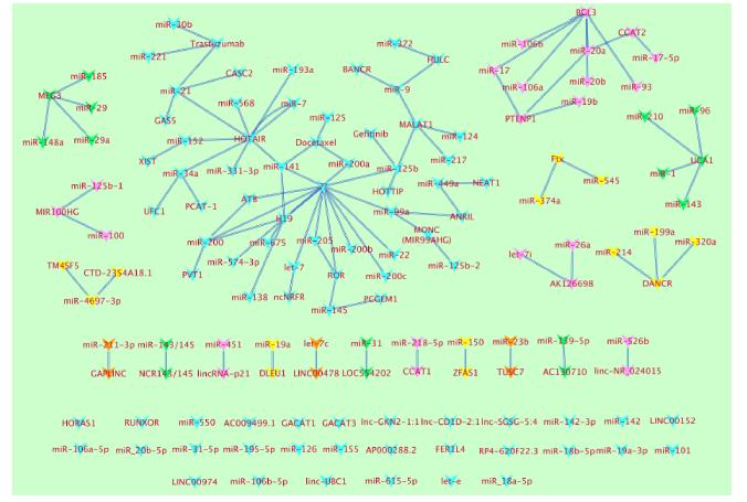
Shannon P, Markiel A, Ozier O, et al. (2003) Cytoscape: a software environment for integrated models of biomolecular interaction networks. Genome Res 13: 2498-2504. doi: 10.1101/gr.1239303
![]() |
[120] | Nair S (2016) Pharmacometrics and systems pharmacology of immune checkpoint inhibitor nivolumab in cancer translational medicine. Adv Mod Oncol Res 2: 18-31. |
[121] |
Elling R, Chan J, Fitzgerald KA (2016) Emerging role of long noncoding RNAs as regulators of innate immune cell development and inflammatory gene expression. Eur J Immunol 46: 504-512. doi: 10.1002/eji.201444558
![]() |
1. | Mo Dong, Haiye Yu, Lei Zhang, Mingzhi Wu, Zhipeng Sun, Dequan Zeng, Ruohan Zhao, Kuruva Lakshmanna, Measurement Method of Plant Phenotypic Parameters Based on Image Deep Learning, 2022, 2022, 1530-8677, 1, 10.1155/2022/7664045 | |
2. | Si Yang, Lihua Zheng, Tingting Wu, Shi Sun, Man Zhang, Minzan Li, Minjuan Wang, High-throughput soybean pods high-quality segmentation and seed-per-pod estimation for soybean plant breeding, 2024, 129, 09521976, 107580, 10.1016/j.engappai.2023.107580 |
Layer Number | Layer Type | Details |
1 | Convolutional Layer | 64 filters of size $3 \times 3 \times 3$, stride of 1, ReLU activation |
2 | Convolutional Layer | 64 filters of size $3 \times 3 \times 64$, stride of 1, ReLU activation |
3 | Max Pooling Layer | $2 \times 2$ kernel, stride of 2 |
4 | Convolutional Layer | 128 filters of size $3 \times 3 \times 64$, stride of 1, ReLU activation |
5 | Convolutional Layer | 128 filters of size $3 \times 3 \times 128$, stride of 1, ReLU activation |
6 | Max Pooling Layer | $2 \times 2$ kernel, stride of 2 |
7 | Convolutional Layer | 256 filters of size $3 \times 3 \times 128$, stride of 1, ReLU activation |
8 | Convolutional Layer | 256 filters of size $3 \times 3 \times 256$, stride of 1, ReLU activation |
9 | Convolutional Layer | 256 filters of size $3 \times 3 \times 256$, stride of 1, ReLU activation |
10 | Max Pooling Layer | $2 \times 2$ kernel, stride of 2 |
11 | Convolutional Layer | 512 filters of size $3 \times 3 \times 256$, stride of 1, ReLU activation |
12 | Convolutional Layer | 512 filters of size $3 \times 3 \times 512$, stride of 1, ReLU activation |
13 | Convolutional Layer | 512 filters of size $3 \times 3 \times 512$, stride of 1, ReLU activation |
14 | Max Pooling Layer | $2 \times 2$ kernel, stride of 2 |
15 | Convolutional Layer | 512 filters of size $3 \times 3 \times 512$, stride of 1, ReLU activation |
16 | Convolutional Layer | 512 filters of size $3 \times 3 \times 512$, stride of 1, ReLU activation |
17 | Convolutional Layer | 512 filters of size $3 \times 3 \times 512$, stride of 1, ReLU activation |
18 | Max Pooling Layer | $2 \times 2$ kernel, stride of 2 |
Flattening | Flatten array resulting from layer 18 into 1-D vector | |
19 | Fully-connected Layer | 4096 units, ReLU activation, Dropout with dropout probability 0.5 |
20 | Fully-connected Layer | 4096 units, ReLU activation, Dropout with dropout probability 0.5 |
21 | Fully-connected Layer | Output layer, 1000 units, Softmax activation |
CNN-HSO | CNN-WSO | CNN-SSO | |
MAD | 1.11 in. | 0.8633 in. | 1.51 sq in. |
$R^2$ | 0.9707 | 0.9444 | 0.9723 |
Prop. Region 1 | 0.610 | 0.665 | 0.565 |
Prop. Region 2 | 0.225 | 0.250 | 0.345 |
Prop. Region 3 | 0.080 | 0.050 | 0.075 |
Prop. Region 4 | 0.085 | 0.035 | 0.015 |
Segmentation-obtained | CNN-HHM | |
MAD | 0.8348 in. | 0.5236 in. |
$R^2$ | 0.9758 | 0.9698 |
Prop. Region 1 | 0.7273 | 0.9057 |
Prop. Region 2 | 0.2290 | 0.0606 |
Prop. Region 3 | 0.0303 | 0.0135 |
Prop. Region 4 | 0.0134 | 0.0202 |
Method | Mean Run Time | Standard Deviation | 95% t-Intervals |
Segmentation | 53.35 | 1.7641 | |
CNN-HSO | 4.67 | 0.4291 | (48.32, 49.04) |
CNN-WSO | 4.71 | 0.4128 | (48.29, 49.00) |
CNN-SSO | 4.86 | 0.3969 | (48.14, 48.85) |
CNN-HHM | 4.85 | 0.4098 | (48.15, 48.86) |