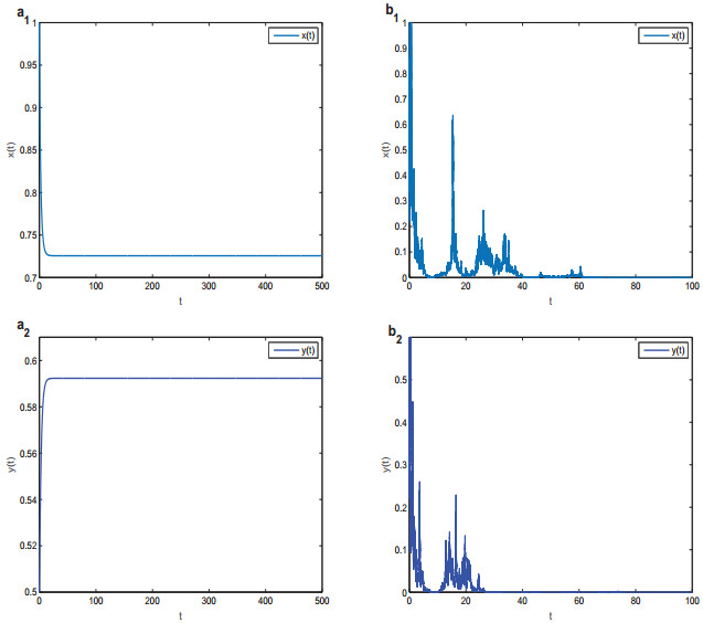
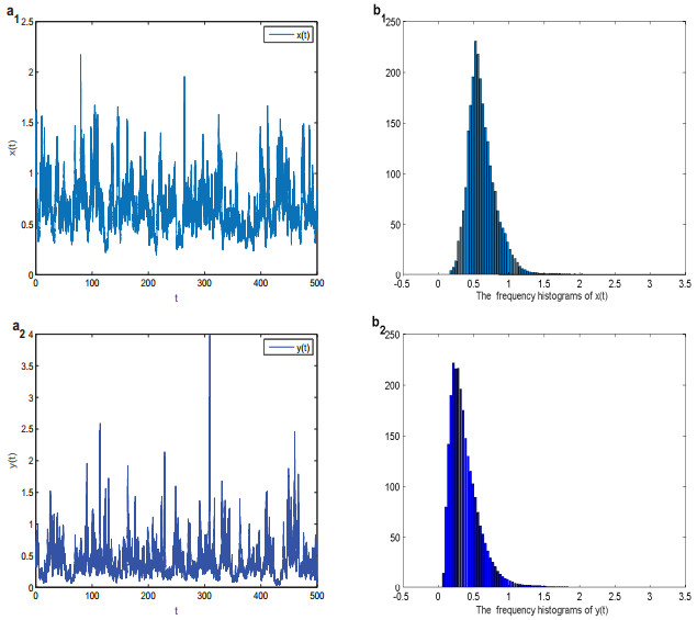
A stochastic two-species competition system with saturation effect and distributed delays is formulated, in which two coupling noise sources are incorporated and every noise source has effect on two species' intrinsic growth rates in nonlinear form. By transforming the two-dimensional system with weak kernel into an equivalent four-dimensional system, sufficient conditions for extinction of two species and the existence of a stationary distribution of the positive solutions to the system are obtained. Our main results show that the two coupling noises play a significant role on the long time behavior of system.
Citation: Jing Hu, Zhijun Liu, Lianwen Wang, Ronghua Tan. Extinction and stationary distribution of a competition system with distributed delays and higher order coupled noises[J]. Mathematical Biosciences and Engineering, 2020, 17(4): 3240-3251. doi: 10.3934/mbe.2020184
A stochastic two-species competition system with saturation effect and distributed delays is formulated, in which two coupling noise sources are incorporated and every noise source has effect on two species' intrinsic growth rates in nonlinear form. By transforming the two-dimensional system with weak kernel into an equivalent four-dimensional system, sufficient conditions for extinction of two species and the existence of a stationary distribution of the positive solutions to the system are obtained. Our main results show that the two coupling noises play a significant role on the long time behavior of system.

| [1] | A. J. Lotka, Elements of Mathematical Biology, Dover, (1924), 167-194. |
| [2] |
V. Volterra, Leçons sur la théorie mathématique de la lutte pour la vie, Bull. Amer. Math. Soc., 42 (1936), 304-305. doi: 10.1090/S0002-9904-1936-06292-0

|
| [3] |
F. J. Ayala, M. E. Gilpin, J. G. Enrenfeld, Competition between species: theoretical models and experimental tests, Theoret. Population Biol., 4 (1973), 331-356. doi: 10.1016/0040-5809(73)90014-2
|
| [4] |
S. Ahmad, On the Nonautonomous Volterra-Lotka Competition Equations, Proc. Amer. Math. Soc., 117 (1993), 199-204. doi: 10.1090/S0002-9939-1993-1143013-3
|
| [5] |
M. L. Zeeman, Extinction in competitive Lotka-Volterra systems, Proc. Amer. Math. Soc., 123 (1995), 87-96. doi: 10.1090/S0002-9939-1995-1264833-2
|
| [6] |
J. Y. Wang, Z. S. Feng, A non-autonomous competitive system with stage structure and distributed delays, Proc. Roy. Soc. Edinburgh Sect. A, 140 (2010), 1061-1080. doi: 10.1017/S0308210509000134
|
| [7] |
F. M. de Oca, L. Perez, Extinction in nonautonomous competitive Lotka-Volterra systems with infinite delay, Nonlinear Anal., 75 (2012), 758-768. doi: 10.1016/j.na.2011.09.009
|
| [8] |
Z. Li, M. A. Han, F. D. Chen, Influence of feedback controls on an autonomous Lotka-Volterra competitive system with infinite delays, Nonlinear Anal. Real World Appl., 14 (2013), 402-413. doi: 10.1016/j.nonrwa.2012.07.004
|
| [9] | J. M. Cushing, Integrodifferential equations and delay models in population dynamics, in Lecture Notes in Biomathematics, Springer Science & Business Media, (2013). |
| [10] | N. Macdonald, Time Lags in Biological Models, in Lecture Notes in Biomathematics, Springer Science & Business Media, (2013). |
| [11] |
X. H. Wang, H. H. Liu, C. L. Xu, Hopf bifurcations in a predator-prey system of population allelopathy with a discrete delay and a distributed delay, Nonlinear Dynam., 69 (2012), 2155-2167. doi: 10.1007/s11071-012-0416-0
|
| [12] |
C. H. Zhang, X. P. Yan, G. H. Cui, Hopf bifurcations in a predator-prey system with a discrete delay and a distributed delay, Nonlinear Anal. Real World Appl., 11 (2010), 4141-4153. doi: 10.1016/j.nonrwa.2010.05.001
|
| [13] |
Q. Liu, D. Q. Jiang, Stationary distribution and extinction of a stochastic predator-prey model with distributed delay, Appl. Math. Lett., 78 (2018), 79-87. doi: 10.1016/j.aml.2017.11.008
|
| [14] |
W. J. Zuo, D. Q. Jiang, X. G. Sun, T. Hayat, A. Alsaedi, Long-time behaviors of a stochastic cooperative Lotka-Volterra system with distributed delay, Phys. A, 506 (2018), 542-559. doi: 10.1016/j.physa.2018.03.071
|
| [15] |
Q. L. Wang, Z. J. Liu, Z. X. Li, R. A. Cheke, Existence and global asymptotic stability of positive almost periodic solutions of a two-species competitive system, Int. J. Biomath., 7 (2014), 1450040. doi: 10.1142/S1793524514500405
|
| [16] | Q. Li, Z. J. Liu, S. L. Yuan, Cross-diffusion induced Turing instability for a competition model with saturation effect, Appl. Math. Comput., 347 (2019), 64-77. |
| [17] |
J. Hu, Z. J. Liu, Incorportating coupling noises into a nonlinear competitive system with saturation effect, Int. J. Biomath., 13 (2020), 2050012. doi: 10.1142/S1793524520500126
|
| [18] | H. C. Chen, C. P. Ho, Persistence and global stability on competition system with time-delay, Tunghai Sci., 5 (2003), 71-99. |
| [19] | Z. J. Liu, R. H. Tan, Y. P. Chen, Modeling and analysis of a delayed competitive system with impulsive perturbations, Rocky Mountain J. Math., 38 (2008), 1505-1523. |
| [20] | R. M. May, Stability and Complexity in Model Ecosystem, Princeton University Press, (2001). |
| [21] |
X. Y. Li, X. R. Mao, Population dynamical behavior of non-autonomous Lotka-Volterra competitive system with random perturbation, Discrete Contin. Dyn. Syst., 24 (2009), 523-545. doi: 10.3934/dcds.2009.24.523
|
| [22] |
F. Y. Wei, C. J. Wang, Survival analysis of a single-species population model with fluctuations and migrations between patches, Appl. Math. Model., 81 (2020), 113-127. doi: 10.1016/j.apm.2019.12.023
|
| [23] |
A. Caruso, M. E. Gargano, D. Valenti, A. Fiasconaro, B. Spagnolo, Cyclic Fluctuations, Climatic Changes and Role of Noise in Planktonic Foraminifera in the Mediterranean Sea, Fluc. Noise Lett., 5 (2005), 349-355. doi: 10.1142/S0219477505002768
|
| [24] |
A. Giuffrida, D. Valenti, G. Ziino, B. Spagnolo, A. Panebianco, A stochastic interspecific competition model to predict the behaviour of Listeria monocytogenes in the fermentation process of a traditional Sicilian salami, Eur. Food Res. Technol., 228 (2009), 767-775. doi: 10.1007/s00217-008-0988-6
|
| [25] |
D. Valenti, G. Denaro, A. La Cognata, B. Spagnolo, A. Bonanno, G. Basilone, et al., Picophytoplankton dynamics in noisy marine environment, Acta Phys. Pol., 43 (2012), 1227-1240. doi: 10.5506/APhysPolB.43.1227
|
| [26] |
Z. W. Cao, W. Feng, X. D. Wen, L. Zu, Stationary distribution of a stochastic predator-prey model with distributed delay and higher order perturbations, Phys. A, 521 (2019), 467-475. doi: 10.1016/j.physa.2019.01.058
|
| [27] |
Q. Liu, D. Q. Jiang, T. Hayat, A. Alsaedi, Long-time behavior of a stochastic logistic equation with distributed delay and nonlinear perturbation, Phys. A, 508 (2018), 289-304. doi: 10.1016/j.physa.2018.05.054
|
| [28] | X. Q. Liu, S. M. Zhong, L. J. Xiang, Asymptotic properties of a stochastic predator-prey model with Bedding-DeAngelis functional response, J. Appl. Math. Comput., 8 (2014), 171-174. |
| [29] | X. R. Mao, Stochastic Differential Equations and their Applications, Horwood Publ, (1997). |
| [30] |
A. Bahar, X. R. Mao, Stochastic delay Lotka-Volterra model, J. Math. Anal. Appl., 292 (2004), 364-380. doi: 10.1016/j.jmaa.2003.12.004
|
| [31] |
C. Lu, X. H. Ding, Persistence and extinction of a stochastic logistic model with delays and impulsive perturbation, Acta Math. Sci. Ser. B, 34 (2014), 1551-1570. doi: 10.1016/S0252-9602(14)60103-X
|
| [32] | R Khasminskii, Stochastic Stability of Differential Equations, Springer Science & Business Media, (2011). |
| [33] |
D. Y. Xu, Y. M. Huang, Z. G. Yang, Existence theorems for periodic Markov process and stochastic functional differential equations, Discrete Contin. Dyn. Syst., 24 (2009), 1005-1023. doi: 10.3934/dcds.2009.24.1005
|
Figures(2)

Jing Hu, Zhijun Liu, Lianwen Wang, Ronghua Tan. Extinction and stationary distribution of a competition system with distributed delays and higher order coupled noises[J]. Mathematical Biosciences and Engineering, 2020, 17(4): 3240-3251. doi: 10.3934/mbe.2020184


 DownLoad: