Spread trend of COVID-19 epidemic outbreak in China: using exponential attractor method in a spatial heterogeneous SEIQR model

Cheng-Cheng Zhu; Jiang Zhu; Cheng-Cheng Zhu; Jiang Zhu

doi:10.3934/mbe.2020174

Mathematical Biosciences and Engineering

2020, Volume 17, Issue 4: 3062-3087. doi: 10.3934/mbe.2020174

Previous Article Next Article

Research article Special Issues

Spread trend of COVID-19 epidemic outbreak in China: using exponential attractor method in a spatial heterogeneous SEIQR model

Cheng-Cheng Zhu ¹,
Jiang Zhu ^{2
,
,}

1.
School of Science, Jiangnan University, Wuxi, Jiangsu 214122, China
2.
School of Mathematics and Statistics, Jiangsu Normal University, Xuzhou, Jiangsu 221116, China

Received: 09 March 2020 Accepted: 08 April 2020 Published: 13 April 2020

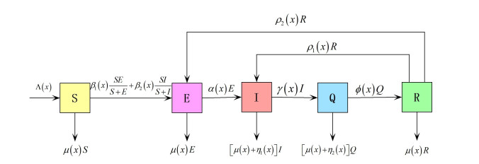
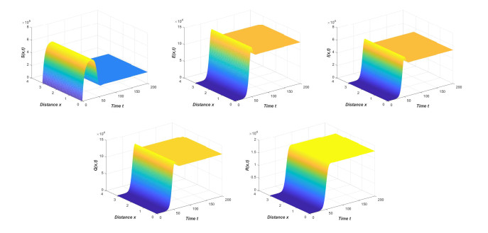
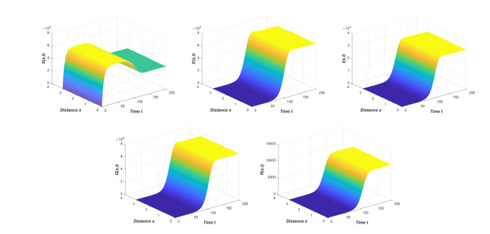
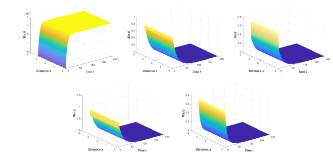
In this paper we introduce a method of global exponential attractor in the reaction-diffusion epidemic model in spatial heterogeneous environment to study the spread trend and long-term dynamic behavior of the COVID-19 epidemic. First, we prove the existence of the global exponential attractor of general dissipative evolution systems. Then, by using the existence theorem, the global asymptotic stability and the persistence of epidemic are discussed. Finally, combine with the official data of the COVID-19 and the national control strategy, some numerical simulations on the stability and global exponential attractiveness of the COVID-19 epidemic are given. Simulations show that the spread trend of the epidemic is in line with our theoretical results, and the preventive measures taken by the Chinese government are effective.
- reaction-diffusion,
- global exponential attractor,
- spatially heterogeneous environment,
- COVID-19
Citation: Cheng-Cheng Zhu, Jiang Zhu. Spread trend of COVID-19 epidemic outbreak in China: using exponential attractor method in a spatial heterogeneous SEIQR model[J]. Mathematical Biosciences and Engineering, 2020, 17(4): 3062-3087. doi: 10.3934/mbe.2020174

Related Papers:

Abstract

In this paper we introduce a method of global exponential attractor in the reaction-diffusion epidemic model in spatial heterogeneous environment to study the spread trend and long-term dynamic behavior of the COVID-19 epidemic. First, we prove the existence of the global exponential attractor of general dissipative evolution systems. Then, by using the existence theorem, the global asymptotic stability and the persistence of epidemic are discussed. Finally, combine with the official data of the COVID-19 and the national control strategy, some numerical simulations on the stability and global exponential attractiveness of the COVID-19 epidemic are given. Simulations show that the spread trend of the epidemic is in line with our theoretical results, and the preventive measures taken by the Chinese government are effective.

References

[1]	S. B. Hsu, F. B. Wang, X. Q. Zhao, Mathematical modeling and analysis of harmful algal blooms in flowing habitats, Math. Biosci. Eng., 16 (2019), 6728-6752. doi: 10.3934/mbe.2019336
[2]	Y. D. Zhang, H. F. Huo, H. Xiang, Dynamics of tuberculosis with fast and slow progression and media coverage, Math. Biosci. Eng., 16 (2019), 1150-1170. doi: 10.3934/mbe.2019055
[3]	F. Li, X. Q. Zhao, Dynamics of a periodic bluetongue model with a temperature-dependent incubation period, SIAM J. Appl. Math., 79 (2019), 2479-2505. doi: 10.1137/18M1218364
[4]	F. Li, X. Q. Zhao, A periodic SEIRS epidemic model with a time-dependent latent period, J. Math. Biol., 78 (2019), 1553-1579. doi: 10.1007/s00285-018-1319-6
[5]	F. Li, J. Liu, X. Q. Zhao, A West Nile Virus model with vertical transmission and periodic time delays, J. Nonlinear Sci., 30 (2020), 449-486. doi: 10.1007/s00332-019-09579-8
[6]	Y. Xing, L. Zhang, X. Wang, Modelling and stability of epidemic model with free-living pathogens growing in the environment, J. Appl. Anal. Comput., 10 (2020), 55-70.
[7]	Z. Xu, C. Ai, Traveling waves in a diffusive influenza epidemic model with vaccination, Appl. Math. Model., 40 (2016), 7265-7280. doi: 10.1016/j.apm.2016.03.021
[8]	C. C. Zhu, W. T. Li, F. Y. Yang, Traveling waves of a reaction-diffusion SIRQ epidemic model with relapse, J. Appl. Anal. Comput., 7 (2017), 147-171.
[9]	C. C. Zhu, J. Zhu, Stability of a reaction-diffusion alcohol model with the impact of tax policy, Comput. Math. Appl., 74 (2017), 613-633. doi: 10.1016/j.camwa.2017.05.005
[10]	B. S. Han, Y. Yang, An integro-PDE model with variable motility, Nonlinear Anal. Real World Appl., 45 (2019), 186-199. doi: 10.1016/j.nonrwa.2018.07.004
[11]	H. F. Huo, S. L. Jing, X. Y. Wang, H. Xiang, Modelling and analysis of an alcoholism model with treatment and effect of twitter, Math. Biosci. Eng., 16 (2019), 3595-3622. doi: 10.3934/mbe.2019179
[12]	Y. Jin, R. Peng, J. Shi, Population dynamics in river networks, J. Nonlinear Sci., 29 (2019), 2501-2545. doi: 10.1007/s00332-019-09551-6
[13]	Z. P. Ma, Spatiotemporal dynamics of a diffusive Leslie-Gower prey-predator model with strong Allee effect, Nonlinear Anal. Real World Appl., 50 (2019), 651-674. doi: 10.1016/j.nonrwa.2019.06.008
[14]	Z. G. Guo, L. P. Song, G. Q. Sun, C. Li, Z. Jin, Pattern dynamics of an SIS epidemic model with nonlocal delay, Int. J. Bifurcat. Chaos, 29 (2019), 1950027. doi: 10.1142/S0218127419500275
[15]	R. Peng, X. Q. Zhao, A reaction-diffusion SIS epidemic model in a time-periodic environment, Nonlinearity, 25 (2012), 1451-1471. doi: 10.1088/0951-7715/25/5/1451
[16]	R. Wu, X. Q. Zhao, A Reaction-Diffusion Model of Vector-Borne Disease with Periodic Delays, J. Nonlinear Sci., 29 (2019), 29-64. doi: 10.1007/s00332-018-9475-9
[17]	F. Y. Yang, W. T. Li, S. Ruan, Dynamics of a nonlocal dispersal SIS epidemic model with Neumann boundary conditions, J. Differential Equations, 267 (2019), 2011-2051. doi: 10.1016/j.jde.2019.03.001
[18]	C. C. Zhu, W. T. Li, F. Y. Yang, Traveling waves in a nonlocal dispersal SIRH model with relapse, Comput. Math. Appl., 73 (2017), 1707-1723. doi: 10.1016/j.camwa.2017.02.014
[19]	L. J. S. Allen, B. M. Bolker, Y. Lou, A. L. Nevai, Asymptotic profiles of the steady states for an SIS epidemic reaction-diffusion model, Discrete Contin. Dyn. Syst., 21 (2008), 1-20. doi: 10.3934/dcds.2008.21.1
[20]	R. Peng, Asymptotic profiles of the positive steady state for an SIS epidemic reaction-diffusion model. Part Ⅰ, J. Differ. Equ., 247 (2009), 1096-1119. doi: 10.1016/j.jde.2009.05.002
[21]	R. Peng, S. Liu, Global stability of the steady states of an SIS epidemic reaction-diffusion model, Nonlinear Anal., 71 (2009), 239-247. doi: 10.1016/j.na.2008.10.043
[22]	R. Peng, F. Yi, Asymptotic profile of the positive steady state for an SIS epidemic reactiondiffusion model: effects of epidemic risk and population movement, Phys. D, 259 (2013), 8-25. doi: 10.1016/j.physd.2013.05.006
[23]	H. Li, R. Peng, Z. A. Wang, On a diffusive SIS epidemic model with mass action mechanism and birth-death effect: analysis, simulations and comparison with other mechanisms, SIAM J. Appl. Math., 78 (2018), 2129-2153. doi: 10.1137/18M1167863
[24]	Y. Tong, C. Lei, An SIS epidemic reaction-diffusion model with spontaneous infection in a spatially heterogeneous environment, Nonlinear Anal. Real World Appl., 41 (2018), 443-460. doi: 10.1016/j.nonrwa.2017.11.002
[25]	P. Song, Y. Lou, Y. Xiao, A spatial SEIRS reaction-diffusion model in heterogeneous environment, J. Differ. Equ., 267 (2019), 5084-5114. doi: 10.1016/j.jde.2019.05.022
[26]	C. C. Zhu, J. Zhu, X. L. Liu, Influence of spatial heterogeneous environment on long-term dynamics of a reaction-diffusion SVIR epidemic model with relapse, Math. Biosci. Eng., 16 (2019), 5897-5922. doi: 10.3934/mbe.2019295
[27]	J. Zhang, Y. Wang, C. K. Zhong, Robustness of exponentially κ-dissipative dynamical systems with perturbation, Discrete Contin. Dyn. Syst. Ser. B, 22 (2017), 3875-3890.
[28]	A. Eden, C. Foias, B. Nicolaenko, R. Temam, Exponential attractors for dissipative evolution equations, Masson, Paris, 1994.
[29]	T. Ma, S. Wang, Phase transition dynamics, Springer Science+Business Media, LLC 2014.
[30]	I. I. Vrabie, C₀ semigroups and application, Elsevier Science B.V., New York, 2003.
[31]	D. Le, Dissipativity and global attractors for a class of quasilinear parabolic systems, Commun. Partial Differ. Equ., 22 (1997), 413-433. doi: 10.1080/03605309708821269
[32]	S. He, S. Tang, L. Rong, A discrete stochastic model of the COVID-19 outbreak: Forecast and control, Math. Biosci. Eng., 17 (2020), 2792-2804. doi: 10.3934/mbe.2020153
[33]	B. Tang, N. L. Bragazzi, Q. Li, S. Tang, Y. Xiao, J. Wu, An updated estimation of the risk of transmission of the novel coronavirus (COVID-19), Infect. Dis. Model, 5 (2020), 248-255.
[34]	Z. Yang, Z. Zeng, K. Wang, S. S. Wong, W. Liang, M. Zanin, et al., Modified SEIR and AI prediction of the epidemics trend of COVID-19 in China under public health interventions, J. Thorac. Dis., (2020), doi: 10.21037/jtd.2020.02.64.
[35]	N. Zhu, D. Zhang, W. Wang, X. Li, B. Yang, J. Song, et al., A novel coronavirus from patients with pneumonia in China, 2019, N. Engl. J. Med., 382 (2020), 727-733. doi: 10.1056/NEJMoa2001017
[36]	Notification of pneumonia outbreak of new coronavirus infection. Available from: http://www.nhc.gov.cn or http://en.nhc.gov.cn.
[37]	Coronavirus disease (COVID-2019) situation reports. Available from: https://www.who.int/emergencies/diseases/novel-coronavirus-2019/situation-reports.
[38]	World Health Statistics, 2013. Available from: http://www.who.int.

Reader Comments

Your name:*

Email:*
© 2020 the Author(s), licensee AIMS Press. This is an open access article distributed under the terms of the Creative Commons Attribution License (http://creativecommons.org/licenses/by/4.0)