Modelling and analysis of HFMD with the effects of vaccination, contaminated environments and quarantine in mainland China

Lei Shi; Hongyong Zhao; Daiyong Wu; Lei Shi; Hongyong Zhao; Daiyong Wu

doi:10.3934/mbe.2019022

Mathematical Biosciences and Engineering

2019, Volume 16, Issue 1: 474-500. doi: 10.3934/mbe.2019022

Previous Article Next Article

Research article

Modelling and analysis of HFMD with the effects of vaccination, contaminated environments and quarantine in mainland China

1.
Department of Mathematics, Nanjing University of Aeronautics and Astronautics, Nanjing, 210016, China
2.
Department of Mathematics, Honghe University, Mengzi 661199, China
3.
Department of Mathematics, Anqing Normal University, Anqing 246133, China

Received: 04 March 2018 Accepted: 13 September 2018 Published: 18 December 2018

Currently, hand, foot, and mouth disease (HFMD) is widespread in mainland China and seriously endangers the health of infants and young children. Recently in mainland China, preventing the spread of the disease has entailed vaccination, isolation measures, and virus clean-up in the contaminated environment. However, quantifying and evaluating the efficacy of these strategies on HFMD remains challenging, especially because relatively little research analyses the impact of EV71 vaccination for this disease. To assess the effectiveness of these strategies, we propose a new mathematical model that considers vaccination, contaminated environment, and quarantine simultaneously. Unlike the previous studies for HFMD, in which the basic reproduction number $R_{0}$ is the only threshold to decide whether the disease is extinct or not, our results show that another threshold value is needed: $\hat{R}_{0} < 1$ ($R_{0}\leq\hat{R}_{0} < 1$) such that disease is extinct; i.e., the disease-free equilibrium is globally asymptotically stable. Moreover, numerical experiments show that our model may have positive equilibriums even if the basic reproduction number $R_{0}$ is less than 1. In designing a new algorithm based on a BP network to estimate the unknown parameters, this proposed model is put forward to individually fit the HFMD reported cases annually in mainland China from 2015 to 2017. At last, the sensitivity analyses and numerical experiments show that increasing the rate of virus clearance, the vaccinated rate of infants and young children, and the quarantined rate of infectious individuals can effectively control the spread of HFMD in mainland China. Nevertheless, it remains difficult to eliminate the disease. Specifically, our results show that the current vaccine measures starting in 2016 have reduced the total number of patients in 2016 and 2017 by 17% and 22%, respectively.
- HFMD,
- vaccination,
- BP network,
- basic reproduction number,
- contaminated environment,
- quarantine
Citation: Lei Shi, Hongyong Zhao, Daiyong Wu. Modelling and analysis of HFMD with the effects of vaccination, contaminated environments and quarantine in mainland China[J]. Mathematical Biosciences and Engineering, 2019, 16(1): 474-500. doi: 10.3934/mbe.2019022

Related Papers:

Abstract

Currently, hand, foot, and mouth disease (HFMD) is widespread in mainland China and seriously endangers the health of infants and young children. Recently in mainland China, preventing the spread of the disease has entailed vaccination, isolation measures, and virus clean-up in the contaminated environment. However, quantifying and evaluating the efficacy of these strategies on HFMD remains challenging, especially because relatively little research analyses the impact of EV71 vaccination for this disease. To assess the effectiveness of these strategies, we propose a new mathematical model that considers vaccination, contaminated environment, and quarantine simultaneously. Unlike the previous studies for HFMD, in which the basic reproduction number $R_{0}$ is the only threshold to decide whether the disease is extinct or not, our results show that another threshold value is needed: $\hat{R}_{0} < 1$ ($R_{0}\leq\hat{R}_{0} < 1$) such that disease is extinct; i.e., the disease-free equilibrium is globally asymptotically stable. Moreover, numerical experiments show that our model may have positive equilibriums even if the basic reproduction number $R_{0}$ is less than 1. In designing a new algorithm based on a BP network to estimate the unknown parameters, this proposed model is put forward to individually fit the HFMD reported cases annually in mainland China from 2015 to 2017. At last, the sensitivity analyses and numerical experiments show that increasing the rate of virus clearance, the vaccinated rate of infants and young children, and the quarantined rate of infectious individuals can effectively control the spread of HFMD in mainland China. Nevertheless, it remains difficult to eliminate the disease. Specifically, our results show that the current vaccine measures starting in 2016 have reduced the total number of patients in 2016 and 2017 by 17% and 22%, respectively.

References

[1]	F. C. Tseng, H. C. Huang, C. Y. Chi, T. L. Lin, C. C. Liu, J. W. Jian, L. C. Hsu, H. S. Wu, J. Y. Yang and Y. W. Chang, Epidemiological survey of enterovirus infections occurring in Taiwan between 2000 and 2005: analysis of sentinel physician surveillance data, J. Med. Virol., 79 (2007), 1850–1860.
[2]	Q. Zhu, Y. Hao, J. Ma, S. Yu and Y. Wang, Surveillance of hand, foot, and mouth disease in mainland China (2008-2009), Biomed. Environ. Sci., 24 (2011), 349–356.
[3]	Chinese Center for Disease Control and Prevention (CCDC), National Public Health Statistical Data. 2018 Available from: http://www.chinacdc.cn/tjsj/fdcrbbg/index.html.
[4]	N. J. Schmidt, E. H. Lennette and H. H. Ho, An apparently new enterovirus isolated from patients with disease of the central nervous system, J. Infect. Dis., 129 (1974), 304–309.
[5]	G. L. Repass, W. C. Palmer and F. F. Stancampiano, Hand, foot and mouth disease: identifying and managing an acute viral syndrome, Clev. Clin. J. Med., 81 (2014), 537–543.
[6]	M. Cabrerizo, D. Tarragó, C. Muñoz-Almagro, A. E. Del, M. Domínguez-Gil, J. M. Eiros, I. López-Miragaya, C. P´erez, J. Reina and A. Otero, Molecular epidemiology of enterovirus 71, coxsackievirus A16 and A6 associated with hand, foot and mouth disease in Spain, Clin. Microbiol. Infec., 20 (2014), O150–O156.
[7]	S. Ljubin-Sternak, V. Slavic-Vrzic, T. Vilibić-Č avlek and I. Gjenero-Margan, Outbreak of hand, foot and mouth disease caused by coxsackie A16 virus in a childcare center in croatia, European Communicable Disease Bulletin, 21 (2011), 9–11.
[8]	N. Sarma, A. Sarkar, A. Mukherjee, A. Ghosh, S. Dhar and R. Malakar, Epidemic of hand, foot and mouth disease in west bengal, india in august, 2007: a multicentric study, Indian J. Dermatol., 54 (2009), 26–30.
[9]	O. M. How,W. S. Chang, M. Anand, P. Yuwana, P. David, C. Daniella, D. S. Sylvia, C. C. Hee, T. P. Hooi and C. M. Jane, Identification and validation of clinical predictors for the risk of neurological involvement in children with hand, foot, and mouth disease in Sarawak, Bmc Infect. Dis., 9 (2009), 3–3.
[10]	T. Fujimoto, M. Chikahira, S. Yoshida, H. Ebira, A. Hasegawa, A. Totsuka and O. Nishio, Outbreak of central nervous system disease associated with hand, foot, and mouth disease in Japan during the summer of 2000: detection and molecular epidemiology of enterovirus 71, Microbiol. Immunol., 46 (2002), 621–627.
[11]	J.Wang, Z. Cao, D. D. Zeng, Q.Wang, X.Wang and H. Qian, Epidemiological analysis, detection, and comparison of space-time patterns of Beijing hand-foot-mouth disease (2008-2012), PLoS One, 9 (2014). Article ID: e92745.
[12]	W. S. Ryu, B. Kang, J. Hong, S. Hwang, J. Kim and D. S. Cheon, Clinical and etiological characteristics of enterovirus 71-related diseases during a recent 2-year period in Korea, J. Clin. Microbiol., 48 (2010), 2490–2494.
[13]	J. Cheng, J.Wu, Z. Xu, R. Zhu, X.Wang, K. Li, L.Wen, H. Yang and H. Su, Associations between extreme precipitation and childhood hand, foot and mouth disease in urban and rural areas in Hefei, China, Sci. Total Environ., 497 (2014), 484–490.
[14]	H. X. Nguyen, C. Chu, H. L. T. Nguyen, H. T. Nguyen, C. M. Do, S. Rutherford and D. Phung, Temporal and spatial analysis of hand, foot, and mouth disease in relation to climate factors: A study in the Mekong Delta region, Vietnam, Sci. Total Environ., 581 (2017), 766–772.
[15]	F. Gou, X. Liu, X. Ren, D. Liu, H. Liu, K. Wei, X. Yang, Y. Cheng, Y. Zheng and X. Jiang, Socioecological factors and hand, foot and mouth disease in dry climate regions: a Bayesian spatial approach in Gansu, China, Int. J. Biometeorol., 61 (2017), 137–147.
[16]	W. Jing, T. Hu, D. Sun, S. Ding, M. J. Carr, W. Xing, S. Li, X. Wang and W. Shi, Epidemiological characteristics of hand, foot, and mouth disease in Shandong, China, 2009-2016, Sci. Rep., 7 (2017). Article ID: 8900.
[17]	Y. Weng, W. Chen, W. He, M. Huang, Y. Zhu and Y. Yan, Serotyping and genetic characterization of hand, foot, and mouth disease (HFMD)-associated enteroviruses of no-ev71 and non-cva16 circulating in fujian, china, 2011-2015, Med. Sci. Monitor, 23 (2017), 2508–2518.
[18]	National Health and Family Planning Commission of the Peoples Republic of China (NHFPC), China Health Statistical Yearbook. 2018 Available from: http://www.moh.gov.cn/zwgk/yqbb3/ejlist.shtml.
[19]	Z. Chang, F. Liu, L. Bin, Z. Wang and L. Zeng, Analysis on surveillance data of hand, foot and mouth disease in China, January - May 2017, Disease Surveillance, 32 (2017), 447–452.
[20]	Y. Cao, Z. Hong, L. Jin, O. U. Jian-Ming and R. Hong, Surveillance of hand, foot and mouth disease in China, 2011-2012, Disease Surveillance, 28 (2013), 975–980.
[21]	J. Sun, Z. Chang, L. Wang and L. Wang, Analysis on the epidemic situation of hand, foot and mouth disease in China in January - March, 2013, Practical Prev. Med., 21 (2014), 183–186.
[22]	J. T. Wu, M. Jit, Y. Zheng, K. Leung and W. Xing, Routine pediatric enterovirus 71 vaccination in China: a cost-effectiveness analysis, Plos Med., 13 (2016). Article ID: e1002013.
[23]	S. Takahashi, Q. Liao, T. P. Van Boeckel, W. Xing, J. Sun, V. Y. Hsiao, C. J. Metcalf, Z. Chang, F. Liu and J. Zhang, Hand, foot, and mouth disease in China: modeling epidemic dynamics of enterovirus serotypes and implications for vaccination, Plos Med., 13 (2016). Article ID: e1001958.
[24]	N. Ziyadi, A male-female mathematical model of human papillomavirus (HPV) in African American population, Math. Biosci. Eng., 14 (2017), 339–358.
[25]	S. Liu, Y. Li, Y. Bi, and Q. Huang, Mixed vaccination strategy for the control of tuberculosis: A case study in China, Math. Biosci. Eng., 14 (2017), 695–708.
[26]	M. L. Manyombe, J. Mbang, J. Lubuma and B. Tsanou, Global dynamics of a vaccination model for infectious diseases with asymptomatic carriers, Math. Biosci., 13 (2016), 813–840.
[27]	Y. C. Wang and F. C. Sung, Modeling the infections for Enteroviruses in Taiwan, Taipei: Institute of Environmental Health (2006). Article ID: 228559790.
[28]	F. C. S. Tiing and J. Labadin, A simple deterministic model for the spread of hand, foot and mouth disease (HFMD) in Sarawak, 2008 Second Asia International Conference on Modelling & Simulation, (2008), 947–952.
[29]	N. Roy, Mathematical modeling of hand-foot-mouth disease: quarantine as a control measure, Int. J. Adv. Sci. Eng. Technol. Res., 1 (2012), 1–11.
[30]	Y. Ma, M. Liu, Q. Hou and J. Zhao, Modelling seasonal HFMD with the recessive infection in Shandong, China, Math. Biosci. Eng., 10 (2013), 1159–1171.
[31]	J.Wang, Y. Xiao and R. A. Cheke, Modelling the effects of contaminated environments on HFMD infections in mainland China, Marriage Fam Rev, 35 (2016), 77–97.
[32]	J. Wang, Y. Xiao and Z. Peng, Modelling seasonal HFMD infections with the effects of contaminated environments in mainland China, Appl. Math. Comput., 271 (2016), 615–627.
[33]	Y. Zhu, B. Xu, X. Lian, W. Lin, Z. Zhou and W. Wang, A hand-foot-and-mouth disease model with periodic transmission rate in Wenzhou, China, Abstr. Appl. Anal., 15 (2014), 1–11.
[34]	Y. Li, J. Zhang and X. Zhang, Modelling and preventive measures of hand, foot and mouth disease (HFMD) in China, Int. J. Environ. Res. Pub. Heal., 11 (2014), 3108–3117.
[35]	Y. Li, L. Wang, L. Pang and S. Liu, The data fitting and optimal control of a hand, foot and mouth disease (HFMD) model with stage structure, Appl. Math. Comput., 276 (2016), 61–74.
[36]	J. Liu, Threshold dynamics for a HFMD epidemic model with periodic transmission rate, Nonlinear Dynam., 64 (2011), 89–95.
[37]	J. Y. Yang, Y. Chen and F. Q. Zhang, Stability analysis and optimal control of a hand-foot-mouth disease (HFMD) model, J. Appl. Math. Comput., 41 (2013), 99–117.
[38]	G. P. Samanta, Analysis of a delayed hand-foot-mouth disease epidemic model with pulse vaccination, Syst. Sci. Control Eng., 2 (2014), 61–73.
[39]	R. Viriyapong and S. Wichaino, Mathematical modeling of hand, foot and mouth disease in the Northern Thailand, Far East J. Math. Sci., 100 (2016), 805–820.
[40]	S. Sharma and G. P. Samanta, Analysis of a hand-foot-mouth disease model, Int. J. Biomath., 10 (2017). Article ID: 1750016.
[41]	P. V. D. Driessche and J. Watmough, Reproduction numbers and sub-threshold endemic equilibria for compartmental models of disease, Math. Biosci., 180 (2002), 29–48.
[42]	W. M. Hirsch, H. Hanisch and J. P. Gabriel, Differential equation models of some parasitic infections: methods for the study of asymptotic behavior, Commun. Pure. Appl. Math., 38 (1985), 733-753.
[43]	X. Zhao, Uniform persistence and periodic coexistence states in infinite-dimensional periodic semiflows with applications, Can. Appl. Math. Q., 3 (1995), 473–495.
[44]	W. Wang and X. Zhao, An epidemic model in a patchy environment, Math. Biosci., 190 (2004), 97–112.
[45]	National Bureau of Statistics of China (NBSC), China Demographic Yearbook of 2013, 2014, 2015, 2016, 2017. 2018 Available from: http://www.stats.gov.cn/tjsj/ndsj/.
[46]	S. Marino, I. B. Hogue, C. J. Ray and D. E. Kirschner, A methodology for performing global uncertainty and sensitivity analysis in systems biology, J. Theor. Biol., 254 (2008), 178–196.
[47]	Y. Xiao, Y. Zhou and S. Tang, Principles of biological mathematics, Xi'an Jiaotong University Press, 2012.
[48]	H. O. Hartley, A. Booker, Nonlinear Least Squares Estimation, Ann. Math. Stat., 36 (1965), 638– 650.
[49]	G. Arminger and B. O. Muth´en, A Bayesian approach to nonlinear latent variable models using the Gibbs sampler and the Metropolis-Hastings algorithm, Psychometrika, 63 (1998), 271–300.
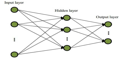
[50]	S. S. Haykin, Neural networks and learning machines, China Machine Press, 2009.

Reader Comments

Your name:*

Email:*
© 2019 the Author(s), licensee AIMS Press. This is an open access article distributed under the terms of the Creative Commons Attribution License (http://creativecommons.org/licenses/by/4.0)